A practical introduction to spatial image filters and morphology, including erosion, dilation, opening, and closing.
1. Image Filtering
Image filtering is a fundamental process in computer vision used to modify or enhance an image. Common applications include denoising, resizing, and sharpening. Filters can be broadly categorized as linear or non-linear.
Linear Filters
A linear filter is a system that modifies an image by applying a linear operator. This operation can be represented as a matrix-vector multiplication. If we "unroll" an image x into a single column vector, the filtered output image y is given by:
$$ y = L x $$
where L is a matrix representing the filter. Two key properties define linear filters:
- Superposition (Additivity): $L(x_1 + x_2) = L(x_1) + L(x_2)$
- Homogeneity (Scaling): $L(a \cdot x) = a \cdot L(x)$
Additionally, most filters used in image processing are shift-invariant (or more accurately, equivariant), meaning that shifting the input image results in a corresponding shift of the output image.
$$ L(\text{shift}(x)) = \text{shift}(y) $$
A system that is both linear and shift-invariant is known as a Linear Time-Invariant (LTI) system, and its operation is equivalent to convolution.
Convolution and Matrix-Vector Multiplication
Convolution is the process of sliding a small matrix, called a kernel or filter, over an image and computing a weighted sum of the pixel values in the neighborhood defined by the kernel.
For an $n \times n$ image convolved with a $k \times k$ kernel, the output size depends on padding.
No Padding (Valid Convolution): The output size is reduced. The resulting output can be represented as a vector in $\mathbb{R}^{(n-k+1)^2 \times n^2}$.
Zero-Padding (Same Convolution): The input image is padded with zeros around the border, typically to preserve the original image dimensions in the output. For a kernel of size $k \times k$, the required padding is $p = (k-1)/2$ on each side (assuming $k$ is odd). The output can be represented as a vector in $\mathbb{R}^{(n+2p-k+1)^2 \times n^2}$.
Correlation vs. Convolution
Correlation and convolution are very similar operations. The key difference lies in how the kernel is applied.
Correlation: The kernel is directly applied to the image neighborhood. The output at $(i, j)$ is a weighted sum of neighbors, finding the similarity between the kernel and the image patch. $$ G(i,j) = \sum_{u=-k}^{k}\sum_{v=-k}^{k} H(u,v) F(i+u, j+v) $$
Convolution: The kernel is first flipped by 180 degrees before being applied. This property is crucial for many mathematical properties, such as the Convolution Theorem. $$ G(i,j) = \sum_{u=-k}^{k}\sum_{v=-k}^{k} H(u,v) F(i-u, j-v) $$
In deep learning, the term "convolution" is often used to refer to what is mathematically a correlation operation, as the kernel weights are learned during training, making the initial flip irrelevant.
Common Filter Types
1. Linear Filters
Box Filter (Averaging Filter): A simple filter where all kernel elements are equal. It is a low-pass filter used for blurring and noise reduction. It is a separable filter, meaning the 2D convolution can be performed as two separate 1D convolutions (one horizontal, one vertical), which is computationally more efficient.
Sharpening Filter: Enhances details and edges in an image. It can be constructed by adding a high-pass version of the image back to the original. Assuming an image can be decomposed into low-frequency (content) and high-frequency (detail) components, a sharpening filter amplifies the detail.
- Let $F$ be the original image and $F_{low}$ be the low-pass filtered (blurred) version.
- The high-pass component is $$ F_{high} = F - F_{low}. $$
- The sharpened image is $$ F_{sharp} = F + \alpha \cdot F_{high} = F + \alpha(F - F_{low}). $$
- This can be rewritten as $(1+\alpha)F - \alpha F_{low}$. The operation can be implemented with a single kernel that combines an identity filter (a pulse at the center) and a scaled negative blurring filter.
2. Non-Linear Filters
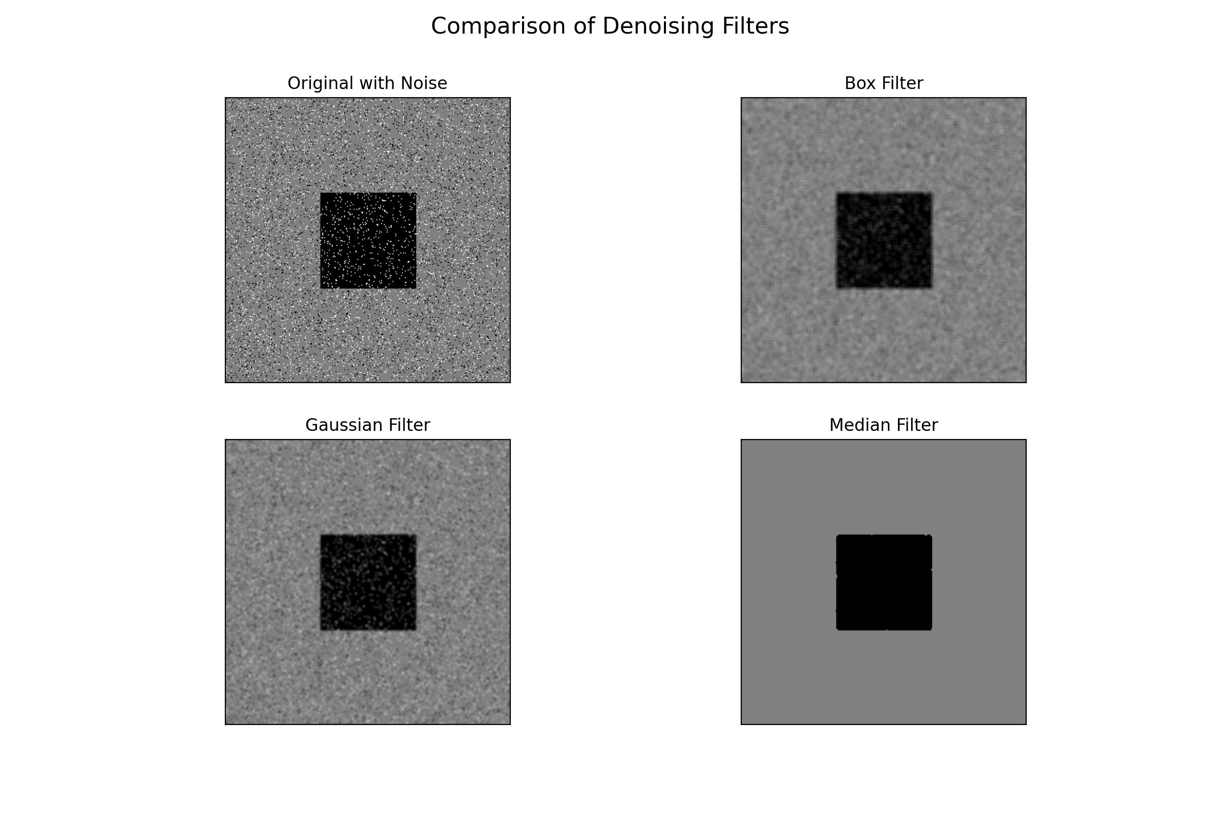
Median Filter: A non-linear filter that is highly effective at removing "salt-and-pepper" noise (random black and white pixels). It operates by sliding a window over the image and replacing the center pixel's value with the median of all pixel values in the window.
- Outlier Robustness: Because the median is used instead of the mean, extreme outlier values (like salt or pepper noise) do not significantly affect the output.
- Edge Preservation: It is better at preserving sharp edges compared to a mean (box) filter of similar size, which tends to blur edges.
Gaussian Filter: The Gaussian filter is a low-pass filter that uses a kernel derived from a 2D Gaussian function. Unlike the box filter which weights all neighbors equally, the Gaussian filter assigns more weight to the central pixel and less to distant neighbors. This results in a smoother, more natural-looking blur and makes it highly effective for removing Gaussian-distributed noise while better preserving edges compared to a simple averaging filter. It is also a separable filter, allowing for efficient computation.
Derivative Filters: These filters are designed to approximate the spatial derivatives of an image. They are fundamental to edge detection and feature extraction.
Prewitt and Sobel Operators: As discussed in Chapter 3, these operators compute an approximation of the image gradient. The Sobel operator, for example, includes a smoothing component (weights of $[1, 2, 1]$) in addition to the differencing component, making it slightly more robust to noise than the Prewitt operator.
Laplacian Operator: This operator approximates the second derivative and is used to find areas of rapid intensity change (edges) and for blob detection. A common 3x3 kernel is $[[0, 1, 0], [1, -4, 1], [0, 1, 0]]$.
Opencv Example
This example demonstrates the effects of different filters on an image with "salt-and-pepper" noise. The Median Filter is non-linear and excels at removing this type of noise, while linear filters like Gaussian and Box filters primarily blur the image.
# Linear and Non-Linear Filtering for Denoising

import cv2
import numpy as np
from matplotlib import pyplot as plt

# 1. Create a sample image and add salt-and-pepper noise
# Using a simple gray image with a black square
image = np.full((300, 300, 3), 128, dtype=np.uint8)
cv2.rectangle(image, (100, 100), (200, 200), (0, 0, 0), -1)

# Add salt-and-pepper noise
salt_pepper = np.random.rand(image.shape[0], image.shape[1])
image[salt_pepper > 0.95] = 255  # Salt
image[salt_pepper < 0.05] = 0    # Pepper

# 2. Apply different filters
# Box filter (Averaging)
box_filtered = cv2.blur(image, (5, 5))

# Gaussian filter
gaussian_filtered = cv2.GaussianBlur(image, (5, 5), 0)

# Median filter
median_filtered = cv2.medianBlur(image, 5)

# 3. Visualize results
titles = ['Original with Noise', 'Box Filter', 'Gaussian Filter', 'Median Filter']
images = [image, box_filtered, gaussian_filtered, median_filtered]

plt.figure(figsize=(12, 8))
for i in range(4):
    plt.subplot(2, 2, i + 1)
    plt.imshow(cv2.cvtColor(images[i], cv2.COLOR_BGR2RGB))
    plt.title(titles[i])
    plt.xticks([]), plt.yticks([])
plt.suptitle("Comparison of Denoising Filters", fontsize=16)
plt.show()
plt.savefig('image-1.jpg', dpi=200)
# The median filter is most effective at removing salt-and-pepper noise while preserving edges,
# whereas the box and Gaussian filters blur the noise along with the image features.
Result:
2. Morphology
Morphological image processing is a collection of non-linear techniques for analyzing and processing geometric structures in an image. It operates by probing an image with a small shape or template known as a structuring element (SE). The SE is positioned at all possible locations in the image and is compared with the corresponding neighborhood of pixels.
Core Operations
The two fundamental morphological operations are dilation and erosion. They are typically applied to binary or grayscale images.
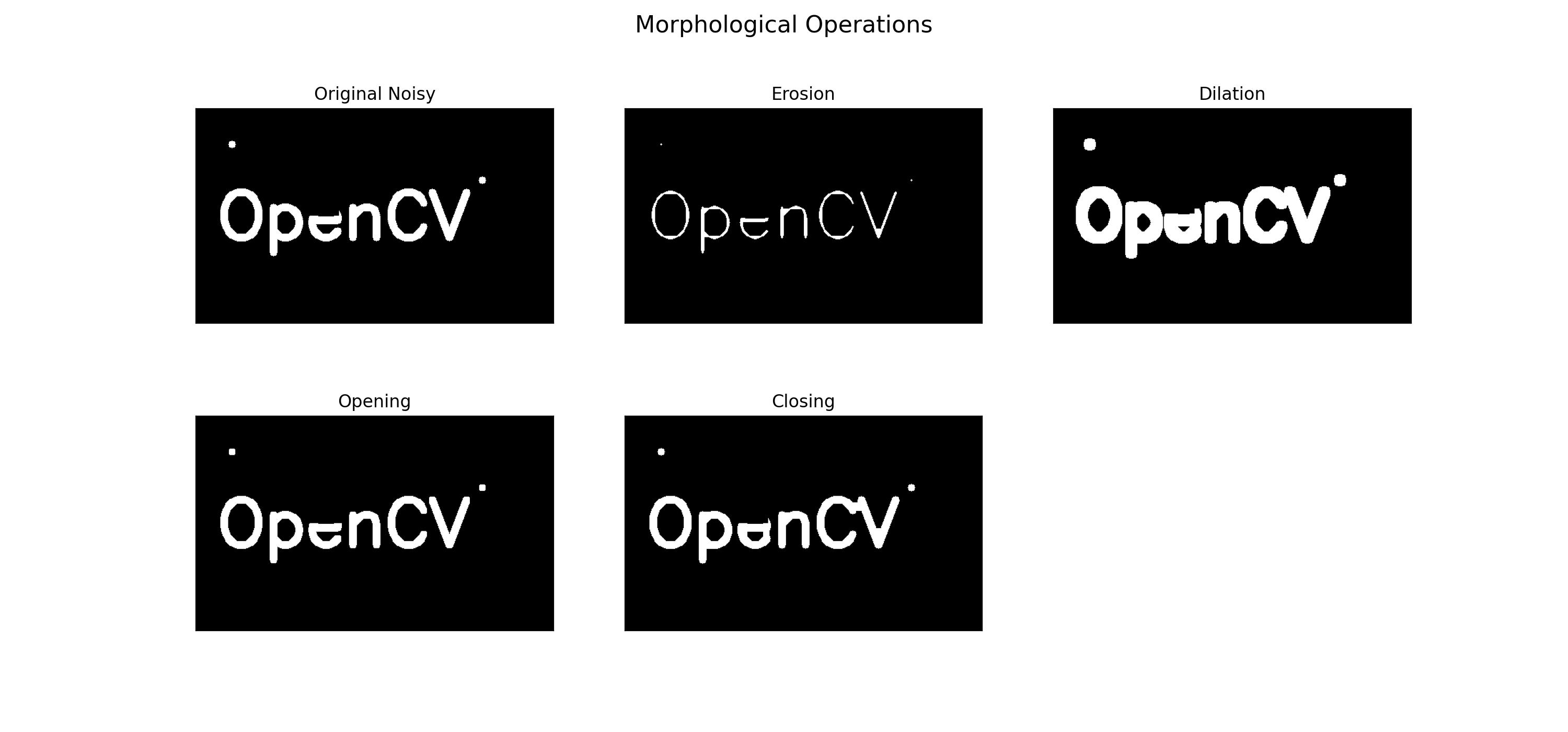
- Dilation: This operation expands or thickens the bright regions of an image. The value of the output pixel is the maximum value of all pixels in the input neighborhood defined by the structuring element. Dilation is used to fill small gaps and connect disjoint objects.
$$ (I \oplus S)(x,y) = \max_{(i,j) \in S} \{I(x-i, y-j)\} $$
- Erosion: This operation shrinks or thins the bright regions. The value of the output pixel is the minimum value of all pixels in the input neighborhood. Erosion is used to remove small-scale noise, break thin connections, and separate touching objects.
$$ (I \ominus S)(x,y) = \min_{(i,j) \in S} \{I(x+i, y+j)\} $$
Compound Operations
By combining dilation and erosion, more complex and useful operations can be created.
- Opening: An erosion followed by a dilation using the same structuring element.
- $I \circ S = (I \ominus S) \oplus S$
- Effect: Opening smooths object contours, breaks narrow connections, and removes small, isolated bright pixels (salt noise). It is "idempotent," meaning applying it multiple times has no further effect. It does not significantly shrink the overall size of large objects.
- Closing: A dilation followed by an erosion using the same structuring element.
- $I \bullet S = (I \oplus S) \ominus S$
- Effect: Closing tends to fill small holes within objects, connect objects that are close together, and smooth contours from the inside. It is also idempotent and is useful for filling in small dark gaps (pepper noise).
Opencv Example
This example shows the four main morphological operations on a noisy binary image. Opening removes small "salt" noise, while Closing fills small "pepper" holes.
# New Chapter: Morphological Image Processing
# Topic: Dilation, Erosion, Opening, and Closing

import cv2
import numpy as np
from matplotlib import pyplot as plt

# 1. Create a noisy binary image
image = np.zeros((300, 500), dtype=np.uint8)
cv2.putText(image, "OpenCV", (30, 180), cv2.FONT_HERSHEY_SIMPLEX, 3, (255), 10)
# Add "pepper" noise (holes)
image[100:150, 150:200] = 0
# Add "salt" noise (small specks)
cv2.circle(image, (400, 100), 5, 255, -1)
cv2.circle(image, (50, 50), 5, 255, -1)

# 2. Define a structuring element and apply operations
kernel = np.ones((7, 7), np.uint8)

# Erosion shrinks bright regions
erosion = cv2.erode(image, kernel, iterations=1)
# Dilation expands bright regions
dilation = cv2.dilate(image, kernel, iterations=1)
# Opening = erosion followed by dilation (removes salt noise)
opening = cv2.morphologyEx(image, cv2.MORPH_OPEN, kernel)
# Closing = dilation followed by erosion (fills pepper holes)
closing = cv2.morphologyEx(image, cv2.MORPH_CLOSE, kernel)

# 3. Visualize results
titles = ['Original Noisy', 'Erosion', 'Dilation', 'Opening', 'Closing']
images = [image, erosion, dilation, opening, closing]

plt.figure(figsize=(15, 7))
for i in range(5):
    plt.subplot(2, 3, i + 1)
    plt.imshow(images[i], 'gray')
    plt.title(titles[i])
    plt.xticks([]), plt.yticks([])
plt.suptitle("Morphological Operations", fontsize=16)
plt.show()
Result: