How image transformations, homographies, feature correspondences, and alignment connect in practical computer vision pipelines.
6. Geometric Transformations
Parametric Transformations
A parametric transformation is a global mapping from one 2D coordinate system to another, defined by a set of parameters. These transformations can be represented by matrices and applied to image coordinates.
- Filtering: Changes the range (pixel values) of an image: $$ g(x) = h(f(x)).$$
- Warping: Changes the domain (pixel coordinates) of an image: $$ g(x) = f(h(x)) .$$
Transformation Hierarchy
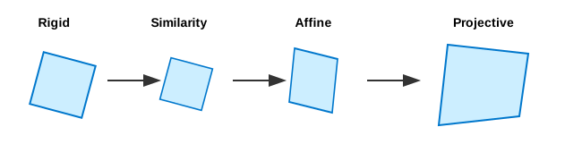
2D transformations form a hierarchy with increasing degrees of freedom (DoF).
Rigid (Euclidean): Preserves distances, angles, and lengths. Composed of rotation and translation. (3 DoF: $\theta, t_x, t_y$)
Similarity: A rigid transformation plus isotropic (uniform) scaling. Preserves angles and ratios of lengths. (4 DoF: $s, \theta, t_x, t_y$)
Affine: A similarity transformation plus shear and non-uniform scaling. Preserves parallelism of lines and ratios of lengths on parallel lines. (6 DoF)
$$ \begin{bmatrix} x' \\ y' \\ 1 \end{bmatrix} = \begin{bmatrix} a & b & t_x \\ c & d & t_y \\ 0 & 0 & 1 \end{bmatrix} \begin{bmatrix} x \\ y \\ 1 \end{bmatrix} $$
Projective (Homography): The most general linear transformation. Preserves straight lines. Parallel lines may converge at a vanishing point. (8 DoF)
$$ \begin{bmatrix} x' \\ y' \\ w' \end{bmatrix} = \begin{bmatrix} h_{11} & h_{12} & h_{13} \\ h_{21} & h_{22} & h_{23} \\ h_{31} & h_{32} & h_{33} \end{bmatrix} \begin{bmatrix} x \\ y \\ 1 \end{bmatrix} $$
Homogeneous Coordinates
Homogeneous coordinates provide a unified framework to represent all these transformations as a single matrix multiplication. A 2D point $(x, y)$ is represented by a 3-vector $[x, y, 1]^T$. A transformation is then a 3x3 matrix multiplication.
The final Cartesian coordinates are found by dividing by the homogeneous coordinate: $$ (x'/w', y'/w'). $$
| Transformation | Degrees of Freedom (DoF) | Properties Preserved |
|---|---|---|
| Translation | 2 | Orientation, Lengths, Angles |
| Rigid (Euclidean) | 3 | Lengths, Angles, Parallelism |
| Similarity | 4 | Angles, Ratios of Lengths, Parallelism |
| Affine | 6 | Parallelism, Ratios of lengths on parallel lines |
| Projective | 8 | Straight Lines |
Opencv Example
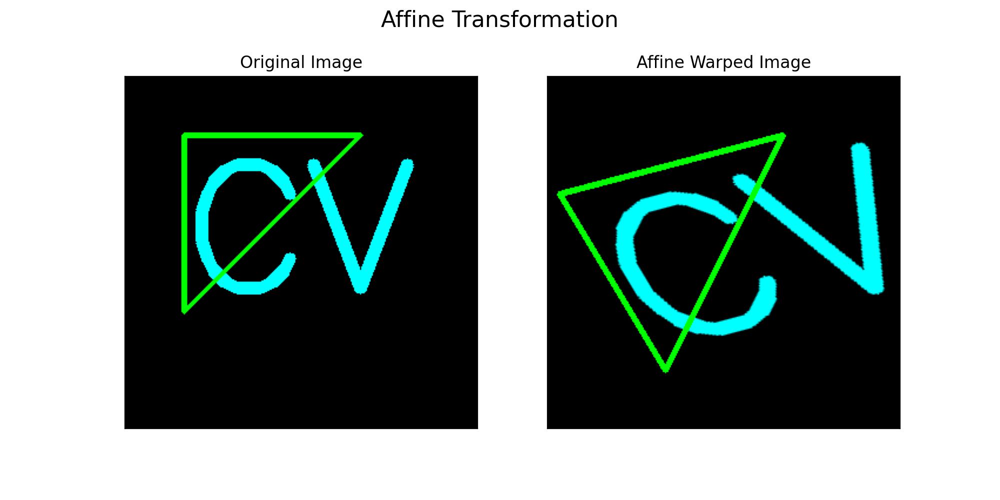
This example applies an Affine Transformation to an image by specifying three pairs of corresponding points.
# Affine Transformation

import cv2
import numpy as np
from matplotlib import pyplot as plt

# 1. Load or create an image
image = np.zeros((300, 300, 3), dtype=np.uint8)
cv2.putText(image, 'CV', (50, 180), cv2.FONT_HERSHEY_SIMPLEX, 5, (255, 255, 0), 10)
rows, cols, _ = image.shape

# 2. Define source and destination points for the transformation
# We will map a triangle to a different triangle
pts1 = np.float32([[50, 50], [200, 50], [50, 200]])
pts2 = np.float32([[10, 100], [200, 50], [100, 250]])

# Get the affine transformation matrix
M = cv2.getAffineTransform(pts1, pts2)

# Apply the transformation
warped_image = cv2.warpAffine(image, M, (cols, rows))

# 3. Visualize results
# Draw the triangles on the images for clarity
cv2.polylines(image, [np.int32(pts1)], True, (0, 255, 0), 3)
cv2.polylines(warped_image, [np.int32(pts2)], True, (0, 255, 0), 3)

plt.figure(figsize=(10, 5))
plt.subplot(1, 2, 1)
plt.imshow(cv2.cvtColor(image, cv2.COLOR_BGR2RGB))
plt.title('Original Image')
plt.xticks([]), plt.yticks([])

plt.subplot(1, 2, 2)
plt.imshow(cv2.cvtColor(warped_image, cv2.COLOR_BGR2RGB))
plt.title('Affine Warped Image')
plt.xticks([]), plt.yticks([])

plt.suptitle("Affine Transformation", fontsize=16)
plt.show()
Result
7. Image Alignment
Image alignment is the process of finding the transformation that maps one image (or set of points) onto another.
Image Warping
Warping applies a geometric transformation to an image. There are two main approaches:
Forward Warping: For each pixel in the source image, compute its destination coordinate in the output image. This can lead to holes (unmapped pixels) and overlaps in the output.
Inverse Warping: For each pixel in the output image, compute its corresponding coordinate in the source image and sample the source image's intensity there. This is generally preferred as it guarantees every output pixel is filled. Since the source coordinate is unlikely to be an integer, interpolation (e.g., bilinear or bicubic) is required.
Correspondence Matching and Least Squares
Given a set of corresponding points between two images, we can estimate the transformation parameters that best align them. For a linear transformation like an Affine transform, this can be formulated as a linear least-squares problem.
An affine transform has 6 unknowns: $$x' = ax + by + c$$ $$y' = dx + ey + f$$
Each pair of corresponding points $(x, y)$ and $(x', y')$ provides two linear equations. With at least 3 point pairs, we can solve for the 6 parameters. This can be written in matrix form as $$At = b$$, where $t$ is the vector of transformation parameters.
$$ \begin{bmatrix} x_1 & y_1 & 1 & 0 & 0 & 0 \\ 0 & 0 & 0 & x_1 & y_1 & 1 \\ x_2 & y_2 & 1 & 0 & 0 & 0 \\ 0 & 0 & 0 & x_2 & y_2 & 1 \\ \vdots & & & & & \vdots \end{bmatrix} \begin{bmatrix} a \\ b \\ c \\ d \\ e \\ f \end{bmatrix} = \begin{bmatrix} x'_1 \\ y'_1 \\ x'_2 \\ y'_2 \\ \vdots \end{bmatrix} $$
When we have more than the minimum number of points (an overdetermined system), we find the least-squares solution that minimizes the sum of squared errors $$ ||At - b||^2. $$
The solution is given by the normal equations: $$ t = (A^T A)^{-1} A^T b $$ The term $(A^T A)^{-1} A^T$ is known as the pseudoinverse of $A$.
Robust Estimation with RANSAC
In practice, point correspondences often contain outliers (incorrect matches) that can severely corrupt the least-squares estimate. The Random Sample Consensus (RANSAC) algorithm is an iterative method to robustly estimate model parameters in the presence of outliers.
The RANSAC procedure is as follows:
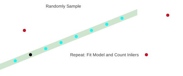
- Sample: Randomly select the minimum number of points required to fit the model (e.g., 3 points for an affine transform, 4 for a homography).
- Compute: Compute the model parameters from this minimal sample.
- Score: Count the number of "inliers"—data points from the entire set that fit the computed model within a certain tolerance.
- Repeat: Repeat steps 1-3 for a fixed number of iterations.
- Choose: Select the model that had the largest number of inliers.
- Refit: Re-estimate the model using all the identified inliers for a more accurate final result.
RANSAC is very effective if the percentage of inliers is reasonably high (e.g., >50%). The number of required iterations depends on the probability of selecting an all-inlier sample.
Opencv Example
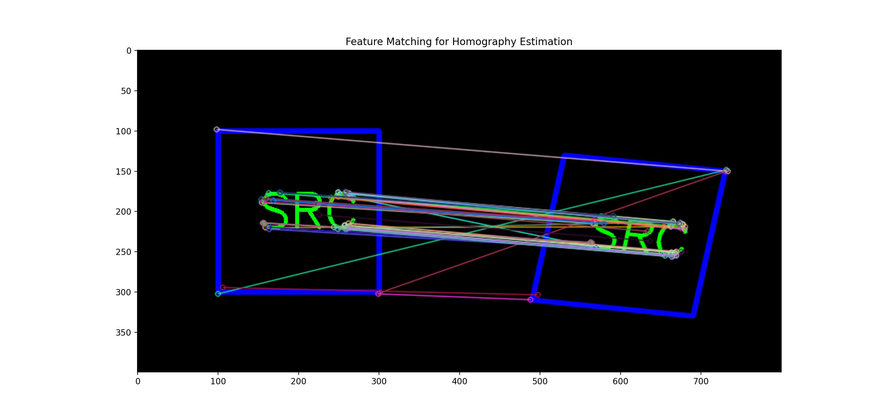
Here, we find a Homography to align two images using ORB feature matching and RANSAC. This is the core of many image stitching and alignment tasks.
# Homography Estimation with Feature Matching

import cv2
import numpy as np
from matplotlib import pyplot as plt

# 1. Create two views of the same scene
# Scene
scene = np.zeros((400, 400, 3), dtype=np.uint8)
cv2.rectangle(scene, (100, 100), (300, 300), (255, 0, 0), 5)
cv2.putText(scene, 'SRC', (150, 220), cv2.FONT_HERSHEY_SIMPLEX, 2, (0, 255, 0), 3)

# Create a second, warped view (e.g., from a different perspective)
M = np.float32([[1, -0.2, 50], [0.1, 0.9, 30]])
warped_scene = cv2.warpAffine(scene, M, (scene.shape[1], scene.shape[0]))

# 2. Find correspondences
# Initialize ORB detector
orb = cv2.ORB_create()
# Find keypoints and descriptors
kp1, des1 = orb.detectAndCompute(scene, None)
kp2, des2 = orb.detectAndCompute(warped_scene, None)

# Use BFMatcher to find the best matches
bf = cv2.BFMatcher(cv2.NORM_HAMMING, crossCheck=True)
matches = bf.match(des1, des2)
# Sort matches by distance
matches = sorted(matches, key=lambda x: x.distance)

# Keep only the best 50 matches for clarity
good_matches = matches[:50]

# 3. Find Homography and visualize
# Extract locations of good matches
src_pts = np.float32([kp1[m.queryIdx].pt for m in good_matches]).reshape(-1, 1, 2)
dst_pts = np.float32([kp2[m.trainIdx].pt for m in good_matches]).reshape(-1, 1, 2)

# Find homography matrix using RANSAC
H, mask = cv2.findHomography(src_pts, dst_pts, cv2.RANSAC, 5.0)

# Draw matches
match_img = cv2.drawMatches(scene, kp1, warped_scene, kp2, good_matches, None, flags=cv2.DrawMatchesFlags_NOT_DRAW_SINGLE_POINTS)

plt.figure(figsize=(15, 7))
plt.imshow(cv2.cvtColor(match_img, cv2.COLOR_BGR2RGB))
plt.title('Feature Matching for Homography Estimation')
plt.show()

# The matrix H can be used to warp the source image to align with the destination image.
Result: