A practical tour of image gradients, Sobel and LoG filters, and the feature detection principles built on top of them.
3. Feature Extraction and Edge Detection
Image Gradients for Edge Detection
Edges in an image are locations with a sharp change in intensity. These changes can be detected by analyzing the image's derivatives. The first derivative of the intensity function will have a local extremum (maximum or minimum) at an edge location. Consequently, the second derivative will have a zero-crossing at that same location.
The gradient of an image $I(x,y)$ is a vector that points in the direction of the greatest intensity increase:
$$ \nabla I = \left[ \frac{\partial I}{\partial x}, \frac{\partial I}{\partial y} \right]^T = [I_x, I_y]^T $$
In a discrete image, derivatives are approximated using finite differences with filter kernels.
Forward difference for $I_x$: $ I(x+1, y) - I(x, y)$, implemented by the kernel $[-1, 1]$.
Forward difference for $I_y$: $ I(x, y+1) - I(x, y)$, implemented by the kernel $[-1, 1]^T$.
The gradient magnitude (intensity) and orientation (direction) are:
Magnitude: $$ ||\nabla I|| = \sqrt{I_x^2 + I_y^2} $$
Orientation: $$ \theta = \tan^{-1}\left(\frac{I_y}{I_x}\right) $$
A significant issue is that differentiation amplifies noise. To mitigate this, it's common practice to first smooth the image (e.g., with a Gaussian filter) and then compute the derivative. Due to the derivative theorem of convolution, this is equivalent to convolving the image with the derivative of the Gaussian kernel:
$$ \frac{\partial}{\partial x}(g * I) = (\frac{\partial g}{\partial x}) * I $$
This combines smoothing and differentiation into a single, efficient step.
Sobel Filter
The Sobel filter is a popular operator for edge detection that approximates the image gradient. It uses two 3x3 kernels to compute the horizontal and vertical derivatives, incorporating a degree of smoothing to reduce noise sensitivity.
Horizontal Gradient ($G_x$): Detects vertical edges.
$$ G_x = \begin{bmatrix} -1 & 0 & +1 \\ -2 & 0 & +2 \\ -1 & 0 & +1 \end{bmatrix} * I $$
Vertical Gradient ($G_y$): Detects horizontal edges.
$$ G_y = \begin{bmatrix} -1 & -2 & -1 \\ 0 & 0 & 0 \\ +1 & +2 & +1 \end{bmatrix} * I $$
The kernels can be seen as combining a differencing operation $[1, 0, -1]$ with a smoothing operation $[1, 2, 1]^T$.
Laplacian of Gaussian (LoG) for Edge Detection
The Laplacian is a 2D isotropic measure of the 2nd spatial derivative of an image. It is defined as: $$ \nabla^2 I = \frac{\partial^2 I}{\partial x^2} + \frac{\partial^2 I}{\partial y^2} $$
Zero-crossings in the Laplacian of a Gaussian-smoothed image correspond to edges. The LoG operator combines these two steps into one:
$$ \nabla^{2} (g * I) = (\nabla^{2} g) * I $$
The $(\nabla^2 g)$ kernel, often called the "Mexican hat" filter, detects edges at a specific scale determined by the Gaussian's standard deviation, $\sigma$.
Seam Carving for Content-Aware Resizing
Seam carving is an algorithm for content-aware image resizing that reduces image size by removing "seams" of low importance rather than by uniform scaling or cropping. A seam is a continuous path of pixels from one edge of the image to the other (e.g., top to bottom).
The process involves:
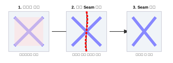
Energy Calculation: An "energy function" is defined to measure the importance of each pixel. A common choice is the gradient magnitude, as pixels with high gradients are part of edges and are perceptually important. $$ e(I) = ||\nabla I|| $$
Optimal Seam Finding: Dynamic programming is used to find the seam with the minimum total energy. Let $M(i, j)$ be the minimum cumulative energy of a seam ending at pixel $(i, j)$. It is calculated recursively: $$ M(i, j) = e(i, j) + \min_{k \in [-1, 0, 1]}M(i-1, j+k) $$
Seam Removal: Once the minimum energy value in the last row is found, the algorithm backtracks to find the entire minimum-energy seam, which is then removed from the image.
This process is repeated to reduce the image to the desired dimensions.
The Canny Edge Detection Pipeline
The Canny edge detector is a multi-stage algorithm widely considered to be the standard in edge detection.
Noise Reduction: The image is first smoothed using a Gaussian filter to suppress noise.
Gradient Calculation: The image gradient intensity and orientation are computed using an operator like Sobel.
Non-Maximum Suppression (NMS): This step thins the wide ridges around edges down to a single pixel width. For each pixel, its gradient magnitude is compared to the two neighbors along its gradient direction. If the pixel's magnitude is not the maximum among the three, it is suppressed (set to zero). This ensures sharp, single-pixel-wide edges.
Hysteresis Thresholding: Two thresholds,
highandweak, are used to link edges.Any pixel with a gradient magnitude above
highis immediately marked as a "strong" edge pixel.Any pixel with a magnitude between
weakandhighis marked as a "weak" edge pixel.Pixels with magnitudes below
weakare suppressed.The final edge map is produced by performing a connectivity analysis: weak pixels that are connected to strong pixels are kept as part of an edge. This allows for the inclusion of faint but legitimate edge sections while discarding isolated noise pixels.
Template Matching
Template matching is a method for finding a specific pattern (template) within a larger image. It works by sliding the template across the search image and computing a similarity score at each location. A common similarity metric is the cross-correlation score. The location with the highest score indicates the best match for the template.
Opencv Example
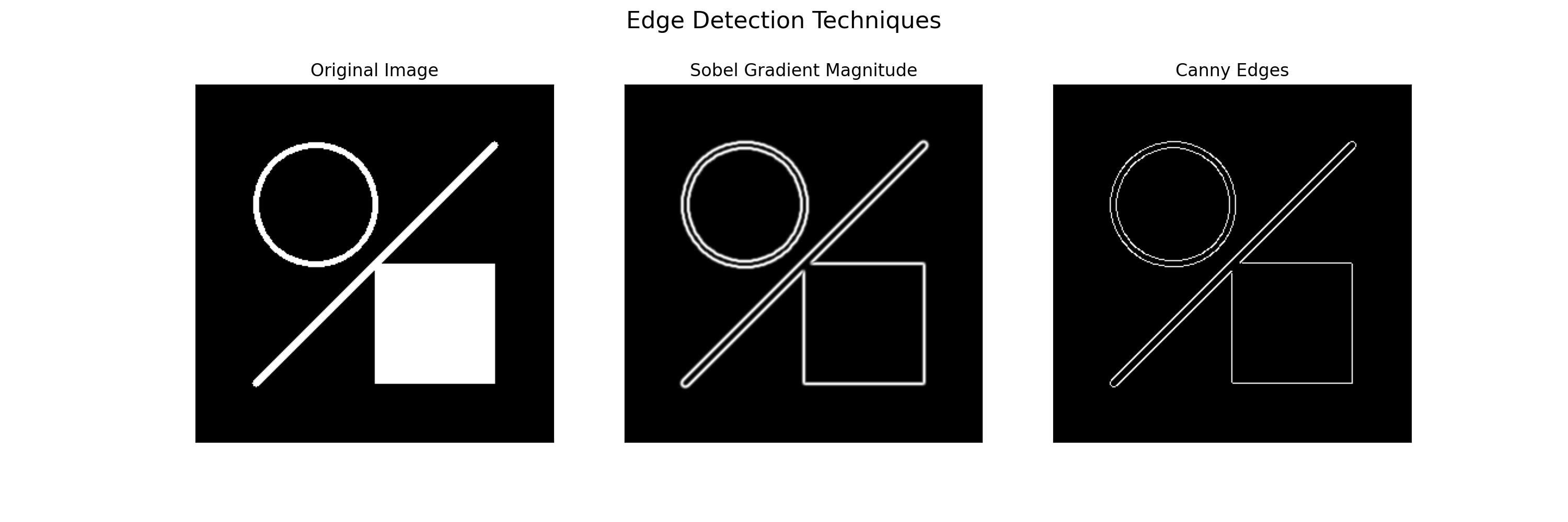
This example compares the Sobel operator for gradient calculation with the more advanced Canny edge detector. Sobel provides gradient magnitude, which can be thresholded, while Canny incorporates non-maximum suppression and hysteresis thresholding for cleaner, single-pixel-wide edges.
# Sobel vs. Canny Edge Detection

import cv2
import numpy as np
from matplotlib import pyplot as plt

# 1. Load an image (or create one)
# Create a sample image with geometric shapes
image = np.zeros((300, 300), dtype=np.uint8)
cv2.circle(image, (100, 100), 50, 255, 3)
cv2.rectangle(image, (150, 150), (250, 250), 255, -1)
cv2.line(image, (50, 250), (250, 50), 255, 5)

# 2. Apply Sobel and Canny detectors
# Sobel operator to find gradients
sobel_x = cv2.Sobel(image, cv2.CV_64F, 1, 0, ksize=5)
sobel_y = cv2.Sobel(image, cv2.CV_64F, 0, 1, ksize=5)
# Compute magnitude and normalize
sobel_magnitude = np.sqrt(sobel_x**2 + sobel_y**2)
sobel_magnitude = np.uint8(255 * sobel_magnitude / np.max(sobel_magnitude))

# Canny edge detector
canny_edges = cv2.Canny(image, threshold1=100, threshold2=200)

# 3. Visualize results
titles = ['Original Image', 'Sobel Gradient Magnitude', 'Canny Edges']
images = [image, sobel_magnitude, canny_edges]

plt.figure(figsize=(15, 5))
for i in range(3):
    plt.subplot(1, 3, i + 1)
    plt.imshow(images[i], cmap='gray')
    plt.title(titles[i])
    plt.xticks([]), plt.yticks([])
plt.suptitle("Edge Detection Techniques", fontsize=16)
plt.show()

# Canny produces clean, thin lines, while Sobel shows the gradient intensity,
# resulting in thick, bright areas around edges.
Results:
4. Resampling and Resizing
Aliasing and the Nyquist Theorem
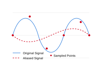
Aliasing is an effect that causes different signals to become indistinguishable when sampled. In images, it manifests as jagged edges, moiré patterns, or other artifacts when an image is downsampled without proper filtering.
The Nyquist-Shannon sampling theorem states that to perfectly reconstruct a signal, the sampling rate must be at least twice the maximum frequency present in the signal ($f_{sample} \ge 2f_{max}$). To prevent aliasing when downsampling an image, we must first remove the high frequencies that would otherwise be misinterpreted. This is achieved by applying a low-pass filter (e.g., a Gaussian blur) before resampling the pixels.
Gaussian and Laplacian Pyramids
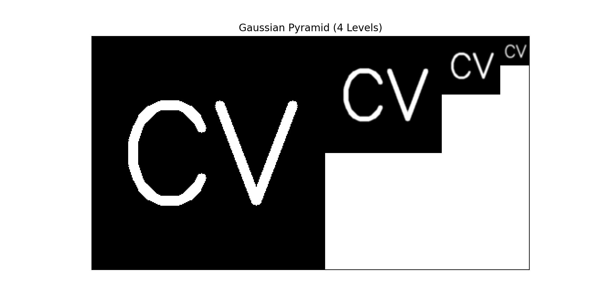
Image pyramids are multi-scale representations of an image, created by repeatedly smoothing and downsampling.
Gaussian Pyramid: A sequence of images where each subsequent level ($G_{i+1}$) is created by Gaussian blurring the previous level ($G_i$) and then downsampling it (typically by a factor of 2). $$ G_{i+1} = \text{Downsample}(\text{GaussianFilter}(G_i)) $$
Laplacian Pyramid: A pyramid that stores the difference between a level in the Gaussian pyramid and its upsampled, blurred predecessor. This captures the high-frequency detail lost between levels. Let $U(G_{i+1})$ be the upsampled version of $G_{i+1}$. $L_i = G_i - U(G_{i+1})$ The original image can be perfectly reconstructed by summing all the levels of the Laplacian pyramid, plus the final level of the Gaussian pyramid.
Interpolation Methods
When resizing an image, interpolation is needed to estimate the pixel values at new coordinates.
Bilinear Interpolation: Estimates a pixel's value by performing linear interpolation in both the horizontal and vertical directions. It considers a 2x2 neighborhood of known pixels.
Bicubic Interpolation: A more advanced method that considers a 4x4 neighborhood of pixels. It fits a cubic polynomial to these pixels, resulting in a smoother, more accurate interpolation than bilinear, but with higher computational cost.
Opencv Example
This code demonstrates the creation of a Gaussian Pyramid, a multi-scale representation of an image created by repeatedly blurring and downsampling.
# Gaussian Pyramid

import cv2
import numpy as np
from matplotlib import pyplot as plt

# 1. Load an image
# To make this runnable without external files, we create a sample image.
# For a real case: image = cv2.imread('your_image.jpg')
image = np.zeros((256, 256, 3), dtype=np.uint8)
cv2.putText(image, 'CV', (30, 180), cv2.FONT_HERSHEY_SIMPLEX, 5, (255, 255, 255), 10)

# 2. Generate the Gaussian pyramid
pyramid_levels = 4
pyramid = [image]
temp_image = image
for i in range(pyramid_levels - 1):
    # Blur and downsample
    temp_image = cv2.pyrDown(temp_image)
    pyramid.append(temp_image)

# 3. Visualize the pyramid
plt.figure(figsize=(10, 5))
# Display images in a row
total_width = sum(img.shape[1] for img in pyramid)
display_image = np.ones((image.shape[0], total_width, 3), dtype=np.uint8) * 255

current_x = 0
for level in pyramid:
    h, w, _ = level.shape
    display_image[0:h, current_x:current_x+w] = level
    current_x += w

plt.imshow(cv2.cvtColor(display_image, cv2.COLOR_BGR2RGB))
plt.title(f'Gaussian Pyramid ({pyramid_levels} Levels)')
plt.xticks([]), plt.yticks([])
plt.show()
Results:
5. Corner Detection
The Intuition Behind Corner Detection
Edges and corners are important features for tasks like matching and tracking. While an edge is characterized by a significant intensity change in one direction, a corner is a point where there is a significant change in all directions. A sliding window analysis reveals this:
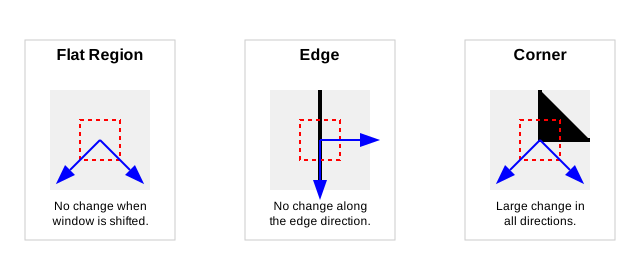
Flat Region: No change when the window is shifted.
Edge: No change when shifted along the edge direction, but a large change when shifted perpendicular to it.
Corner: A large change when the window is shifted in any direction.
Harris Corner Detector
The Harris corner detector formalizes this intuition. It analyzes the change in intensity caused by a small shift $(u, v)$.
The sum of squared differences (SSD) error $E(u, v)$ is:
$$ E(u,v) = \sum_{x,y \in W} [I(x+u, y+v) - I(x,y)]^2
$$
where W is the sliding window.
Using a first-order Taylor expansion, this can be approximated as:
$$ E(u,v) \approx \sum_{W} [I_x u + I_y v]^2 = [u, v] \left( \sum_{W} \begin{bmatrix} I_x^2 & I_x I_y \\ I_x I_y & I_y^2 \end{bmatrix} \right) \begin{bmatrix} u \\ v \end{bmatrix} $$
This can be written compactly as: $$ E(u,v) \approx [u, v] H \begin{bmatrix} u \\ v \end{bmatrix} $$ where $H$ is the structure tensor or Harris matrix, which sums the gradient information over the window $W$.
The behavior of $E(u,v)$ is determined by the eigenvalues, $\lambda_1$ and $\lambda_2$, of $H$.
Flat Region: Both $\lambda_1$ and $\lambda_2$ are small.
Edge: One eigenvalue is large, and the other is small ($\lambda_1 \gg \lambda_2$ or $\lambda_2 \gg \lambda_1$).
Corner: Both $\lambda_1$ and $\lambda_2$ are large.
Since computing eigenvalues is expensive, the Harris detector uses a response function $R$: $$ R = \det(H) - k \cdot (\text{trace}(H))^2 = \lambda_1 \lambda_2 - k(\lambda_1 + \lambda_2)^2 $$ where $k$ is an empirical constant (typically 0.04-0.06). A pixel is classified as a corner if its response $R$ is above a certain threshold.
Equivariance vs. Invariance
These terms describe how a function's output behaves under a transformation of its input.
Equivariance: A function $f$ is equivariant to a transformation $T$ if transforming the input is equivalent to transforming the output: $$ T(f(x)) = f(T(x)) $$. A corner detector is ideally equivariant to geometric transformations like rotation; if an image is rotated, the detected corner locations should also rotate.
Invariance: A function $f$ is invariant to a transformation $T$ if the output does not change when the input is transformed: $$ f(x) = f(T(x) $)$. A feature descriptor is ideally invariant to photometric transformations like brightness changes; the descriptor should remain the same even if the lighting changes.
Blob Detection with Laplacian of Gaussian (LoG)
Blobs are image regions that are roughly circular and differ in properties (e.g., brightness or color) from their surroundings. The Laplacian of Gaussian (LoG) operator is an excellent blob detector. The LoG filter responds strongly to regions that match its size (determined by $\sigma$) and have a sharp intensity change. To find blobs of unknown sizes, one can apply LoG filters at multiple scales and look for local extrema in the 3D scale-space volume. The scale that gives the maximum response corresponds to the characteristic scale of the blob.
Opencv Example
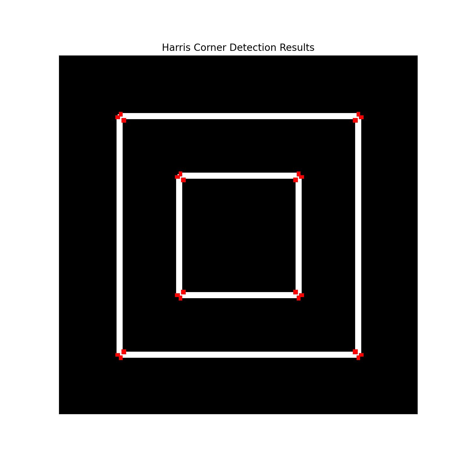
The code finds corners in an image using the Harris Corner Detection algorithm and marks them with circles.
# Harris Corner Detector

import cv2
import numpy as np
from matplotlib import pyplot as plt

# 1. Load an image or create a synthetic one
# Create a synthetic image with corners
image = np.zeros((300, 300), dtype=np.uint8)
cv2.rectangle(image, (50, 50), (250, 250), 255, 3)
cv2.rectangle(image, (100, 100), (200, 200), 255, 3)
image_color = cv2.cvtColor(image, cv2.COLOR_GRAY2BGR) # For drawing colored circles

# 2. Apply Harris Corner Detector
gray = np.float32(image)
# harris_corners = cv2.cornerHarris(src, blockSize, ksize, k)
harris_corners = cv2.cornerHarris(gray, 2, 3, 0.04)

# Dilate the corner image to make the corners more visible
harris_corners = cv2.dilate(harris_corners, None)

# 3. Threshold and visualize the corners
# Mark the detected corners on the original image
image_color[harris_corners > 0.01 * harris_corners.max()] = [0, 0, 255] # Red

plt.figure(figsize=(8, 8))
plt.imshow(cv2.cvtColor(image_color, cv2.COLOR_BGR2RGB))
plt.title('Harris Corner Detection Results')
plt.xticks([]), plt.yticks([])
plt.show()
Results: