From camera projection to stereo correspondence, deriving the epipolar geometry used to recover 3D structure from two views.
8. Camera Models
The Pinhole Camera Model (Camera Obscura)
The simplest model for a camera is the pinhole camera. It consists of a light-proof box with a tiny aperture (the pinhole) on one side and an image plane (film or sensor) on the other. Light rays from a 3D point in the world pass through the pinhole and project an inverted image onto the image plane.
The relationship between a 3D world point $(X, Y, Z)$ and its projected 2D image coordinates $(x, y)$ is given by similar triangles:
$$x = f \frac{X}{Z}$$
$$y = f \frac{Y}{Z}$$
where f is the focal length, the distance from the pinhole (center of projection) to the image plane.
Aperture Size: A smaller aperture produces a sharper image but lets in less light. However, making the aperture too small leads to diffraction effects, which blur the image.
Lens: A lens is used to gather more light, allowing for a larger aperture while still focusing the light onto the image plane. However, lenses can introduce distortions. The circle of confusion describes the blur spot created by a lens for points that are not perfectly in focus.
Projection Models
Using homogeneous coordinates, the mapping from 3D world points to 2D image points can be expressed as a matrix multiplication.
Perspective Projection: This is the standard model described above. A 3D point $[X, Y, Z, 1]$ is mapped to a 2D image point $[x, y, 1]$.
$$ \begin{bmatrix} fX \\ fY \\ Z \end{bmatrix} = \begin{bmatrix} f & 0 & 0 & 0 \\ 0 & f & 0 & 0 \\ 0 & 0 & 1 & 0 \end{bmatrix} \begin{bmatrix} X \\ Y \\ Z \\ 1 \end{bmatrix} $$
After dividing by the third coordinate (Z), we get the image coordinates $(fX/Z, fY/Z)$.Orthographic Projection: A simplified model that approximates perspective projection when the camera is far from the object (like a telephoto lens). It assumes all rays are parallel and simply drops the Z coordinate. It does not model perspective effects like objects appearing smaller with distance.
$$ \begin{bmatrix} x \\ y \\ 1 \end{bmatrix} = \begin{bmatrix} 1 & 0 & 0 & 0 \\ 0 & 1 & 0 & 0 \\ 0 & 0 & 0 & 1 \end{bmatrix} \begin{bmatrix} X \\ Y \\ Z \\ 1 \end{bmatrix} $$
Camera Parameters
The full camera projection matrix $P$ maps 3D world coordinates to 2D pixel coordinates and can be decomposed into two main components: extrinsic and intrinsic parameters.
1. Extrinsic Parameters $[R|t]$: These define the camera's position and orientation in the world. They specify the rigid transformation from 3D world coordinates to 3D camera coordinates.
Rotation $R$: A 3x3 rotation matrix.
Translation $t$: A 3x1 translation vector representing the camera's position.
2. Intrinsic Matrix K: These parameters are internal to the camera and define how it projects 3D camera coordinates onto the 2D image plane in pixel units.
$$ K = \begin{bmatrix} \alpha_x & s & c_x \\ 0 & \alpha_y & c_y \\ 0 & 0 & 1 \end{bmatrix} $$
Focal Lengths ($\alpha_x, \alpha_y$): Focal length $f$ scaled by the pixel size: $\alpha_x = f \cdot s_x$, $\alpha_y = f \cdot s_y$.
Principal Point ($c_x, c_y$): The coordinates of the point where the optical axis intersects the image plane (the image center).
Skew Coefficient ($s$): Accounts for any non-perpendicularity between the x and y sensor axes. This is almost always zero for modern cameras.
The full projection equation is:
$$ \mathbf{x}_\text{image} = P \mathbf{X}_\text{world} = K [R|t] \mathbf{X}_\text{world} $$
Opencv Example
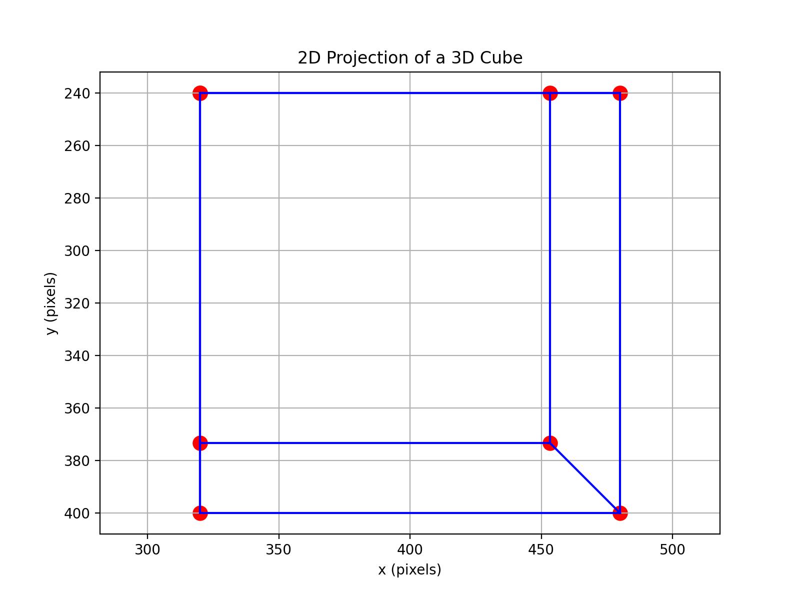
This example demonstrates the core concept of a camera matrix by manually projecting 3D points of a cube onto a 2D image plane.
# Projecting 3D Points to a 2D Image Plane

import numpy as np
import matplotlib.pyplot as plt

# 1. Define camera parameters and 3D points
# Camera Intrinsic Matrix K (a simple example)
f = 800 # Focal length
cx, cy = 320, 240 # Principal point
K = np.array([[f, 0, cx],
              [0, f, cy],
              [0, 0, 1]])

# Camera Extrinsic Parameters [R|t] (camera looks along Z-axis)
R = np.identity(3) # No rotation
t = np.array([[0], [0], [5]]) # Camera is 5 units away from origin

# Define a 3D cube (8 vertices)
cube_points_3d = np.array([
    [0, 0, 0], [1, 0, 0], [1, 1, 0], [0, 1, 0],
    [0, 0, 1], [1, 0, 1], [1, 1, 1], [0, 1, 1]
]).T # Transpose to get 3xN

# 2. Project the 3D points to the 2D image plane
# First, transform from world to camera coordinates
points_cam_coord = R @ cube_points_3d + t

# Then, project to 2D using the intrinsic matrix K
# The projection equation is: x_img = K * X_cam
projected_points_homogeneous = K @ points_cam_coord

# Convert from homogeneous to Cartesian coordinates by dividing by the last component (Z)
projected_points_2d = projected_points_homogeneous[:2, :] / projected_points_homogeneous[2, :]

# 3. Visualize the 2D projection
plt.figure(figsize=(8, 6))
# Plot projected points
plt.scatter(projected_points_2d[0, :], projected_points_2d[1, :], c='red', s=100)

# Draw lines to form the cube
edges = [[0, 1], [1, 2], [2, 3], [3, 0], [4, 5], [5, 6],
         [6, 7], [7, 4], [0, 4], [1, 5], [2, 6], [3, 7]]
for edge in edges:
    p1 = projected_points_2d[:, edge[0]]
    p2 = projected_points_2d[:, edge[1]]
    plt.plot([p1[0], p2[0]], [p1[1], p2[1]], 'b-')

plt.title('2D Projection of a 3D Cube')
plt.xlabel('x (pixels)')
plt.ylabel('y (pixels)')
plt.gca().invert_yaxis() # Image coordinates usually have y-axis pointing down
plt.grid(True)
plt.axis('equal')
plt.show()
Result:
9. Panoramas
Creating Panoramas with Homographies
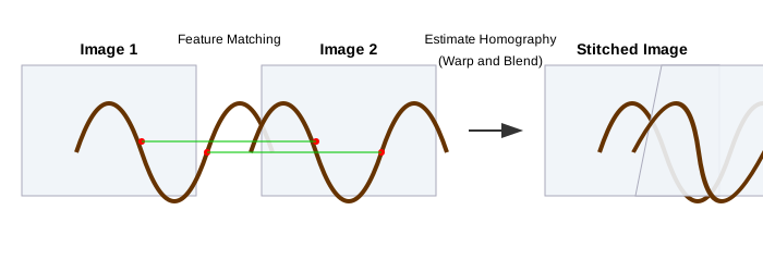
A panorama is a wide-angle image created by stitching together multiple overlapping photographs. If the images are taken by rotating the camera about its optical center (COP), the relationship between any two overlapping images is a homography (a 2D projective transformation).
The basic procedure is:
- Acquire Images: Take a sequence of overlapping photos by rotating the camera from a fixed position (ideally on a tripod).
- Feature Detection & Matching: Detect keypoints (e.g., SIFT, ORB) and find correspondences between adjacent images.
- Homography Estimation: For each pair of overlapping images, use a robust algorithm like RANSAC to compute the homography matrix
Hthat aligns them. - Warping and Compositing: Warp all images into a common reference frame (e.g., the frame of the center image) using the computed homographies. Then, blend the overlapping regions to create a seamless final mosaic.
Spherical Projection
For very wide-angle or 360° panoramas, projecting onto a single plane causes extreme distortion at the edges. A better approach is to project the images onto a common spherical surface.
The process is:
Warp to Sphere: Each image is warped from its planar coordinates $(x', y')$ to spherical coordinates $(\theta, \phi)$ using the camera's focal length $f$.
- Convert pixel coordinates to 3D rays: $$ (x, y, z) = (x' - c_x, y' - c_y, f).$$
- Normalize to unit sphere: $$(\hat{x}, \hat{y}, \hat{z}) = (x, y, z) / \sqrt{x^2+y^2+z^2}.$$
- Convert to spherical angles: $$\theta = \text{atan2}(\hat{y}, \hat{x}), \phi = \text{acos}(\hat{z}). $$
Align on Sphere: The images are aligned on the spherical surface.
Render Panorama: The final panoramic image is rendered by projecting a portion of the sphere back onto a cylindrical or planar surface.
10. Single View Modeling
Single view geometry involves inferring 3D properties of a scene from a single 2D image by exploiting the constraints of projective geometry.
Point-Line Duality in 2D Projective Space
In 2D homogeneous coordinates, there is a beautiful symmetry between points and lines.
- A line $l$ is represented by a 3-vector $(a, b, c)$. A point $p = (x, y, 1)$ lies on the line if $p^T l = ax + by + c = 0$.
- The line passing through two points $p_1$ and $p_2$ is given by their cross product: $l = p_1 \times p_2$.
- The point of intersection of two lines $l_1$ and $l_2$ is given by their cross product: $p = l_1 \times l_2$.
This duality means that any theorem about points and lines can be restated by swapping the words "point" and "line" to get another valid theorem.
Ideal Points (Points at Infinity): In homogeneous coordinates, a point with its last coordinate equal to zero, $p = (x, y, 0)$, represents a point at infinity in the direction of the vector $(x, y)$. It is the intersection point of a set of parallel lines.
The Line at Infinity ($l_\infty$): The line represented by the vector $(0, 0, 1)$. All ideal points lie on this line.
Vanishing Points and Lines
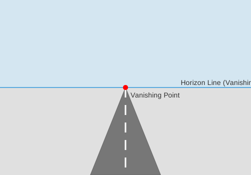
Vanishing Point: The projection of a point at infinity onto the image plane. All parallel lines in 3D space appear to converge at a single vanishing point in the image. The vanishing point for a set of lines with direction
dis given by $v = Pd$, wherePis the camera matrix.Vanishing Line (Horizon): The projection of a line at infinity from a 3D plane onto the image plane. All vanishing points corresponding to directions on that plane will lie on this vanishing line. For example, the horizon line in an image is the vanishing line of the ground plane.
Measuring Height from a Single View
Projective geometry allows us to make metric measurements from a single image if some references are known. The cross-ratio is a fundamental projective invariant. For any four collinear points A, B, C, D, their cross-ratio is preserved under projective transformation.
Using this principle, we can measure the height of an object in a scene:
Identify the vertical vanishing point ($v_z$) by finding the intersection of two or more vertical parallel lines in the image.
Identify four key collinear points in the image: the base of the object (B), its top (T), the base of a reference object of known height (b), and its top (t). These points should lie on lines that converge to the same vanishing point.
Using the cross-ratio and the known reference height, the unknown object's height (H) can be calculated. The formula involves computing the cross-product of lines defined by these points and the vanishing point.
11. Stereo Vision
Stereo vision uses two or more cameras to infer depth from a scene, mimicking human binocular vision.
Disparity and Depth Perception
When two cameras view the same scene from slightly different positions, a 3D point is projected to different locations in the two images. The difference in these image locations is called disparity.
For a simple stereo setup with two parallel cameras separated by a baseline $T$, the relationship between disparity $d = x_l - x_r$ and depth $Z$ is: $$ Z = \frac{f \cdot T}{d} $$
where $f$ is the focal length. Depth is inversely proportional to disparity: large disparity means the object is close, while small disparity means it is far away.
Epipolar Geometry
Epipolar geometry describes the geometric constraints between two views of a scene.
Epipoles ($e_l, e_r$): The projection of one camera's center into the other camera's image plane.
Epipolar Line: For a point
p_lin the left image, the corresponding pointp_rin the right image must lie on a specific line called the epipolar line. This line is the projection of the ray from the left camera's center throughp_l.Epipolar Constraint: This powerful constraint reduces the search for a corresponding point from a 2D area to a 1D line, dramatically simplifying the stereo matching problem.
Stereo Matching as Energy Minimization
Finding the correct disparity for each pixel is the core challenge of stereo vision. This is often formulated as an energy minimization problem. The goal is to find a disparity map d that minimizes a total energy function E(d).
$$ E(d) = E_{data}(d) + \lambda E_{smooth}(d) $$
- Data Term ($E_{data}$): This term penalizes poor matches. It measures the dissimilarity between a pixel patch in the left image and the corresponding patch (shifted by disparity
d) in the right image. A common metric is the Sum of Squared Differences (SSD). - Smoothness Term ($E_{smooth}$): This term enforces the assumption that nearby pixels should have similar disparities, reflecting the fact that surfaces are generally smooth. It penalizes large differences in disparity between neighboring pixels.
The Fundamental Matrix and Camera Calibration
The Fundamental Matrix F is a 3x3 matrix that algebraically encapsulates the epipolar geometry. For any pair of corresponding points $p$ in the left image and $q$ in the right image (in homogeneous coordinates), they must satisfy the epipolar constraint:
$$ q^T F p = 0
$$
The Fundamental Matrix has 7 degrees of freedom and can be computed from at least 7 point correspondences.
If the cameras are calibrated (i.e., their intrinsic matrices $K_l, K_r$ are known), the geometry is described by the Essential Matrix E, which relates to the camera's relative pose (rotation R and translation t):
$$ E = [t]_{\times} R
$$
where $[t]*{\times}$ is the skew-symmetric matrix representation of the cross product with t. The Fundamental and Essential matrices are related by:
$$F = (K_r^{-1})^T E K_l^{-1}$$
Stereo Rectification: To simplify matching, stereo images are often rectified. This process warps both images so that the epipoles are moved to infinity and all epipolar lines become horizontal and aligned in the same rows. This reduces the correspondence search to a simple horizontal scan along the same row in the other image.
Stereo Rectification
Stereo Rectification is a crucial preprocessing step that transforms a pair of stereo images such that their corresponding epipolar lines become collinear and horizontal. This is achieved by applying a projective transformation (a homography) to each image.
- Purpose: The primary goal is to simplify the correspondence problem. After rectification, the search for a matching point for pixel
(x, y)in the left image is reduced from a 2D search in the right image to a 1D horizontal scan along the same rowy. - Process: The transformation matrices are computed from the fundamental matrix
Fand the camera intrinsic parameters. The process effectively rotates the virtual camera planes to be coplanar and aligns their scanlines.
Disparity Map Refinement
The raw disparity map computed by a stereo matching algorithm often contains errors and artifacts. Refinement techniques are used to improve its quality.
Left-Right Consistency Check: This is a powerful method for detecting occlusions and mismatches. A disparity
dcalculated for a point $p_l$ in the left image is considered valid only if the corresponding point in the right image, $p_r$, when matched back to the left image, results in a disparity ofd. Points that fail this check are marked as invalid, as they are typically occluded in one of the views.Sub-pixel Estimation: Matching algorithms initially produce integer-valued disparities. To achieve higher precision, the matching cost function (e.g., SSD) around the best integer disparity is analyzed. By fitting a curve (like a parabola) to the cost values at the integer disparity and its two neighbors, the true minimum can be estimated at a sub-pixel location.
Hole Filling and Filtering: Invalid pixels identified by the consistency check create "holes" in the disparity map. These are often filled by propagating disparity values from nearby valid pixels. Finally, a median filter or a more advanced bilateral filter can be applied to the disparity map to smooth out noise while preserving sharp depth discontinuities at object boundaries.
Opencv Example
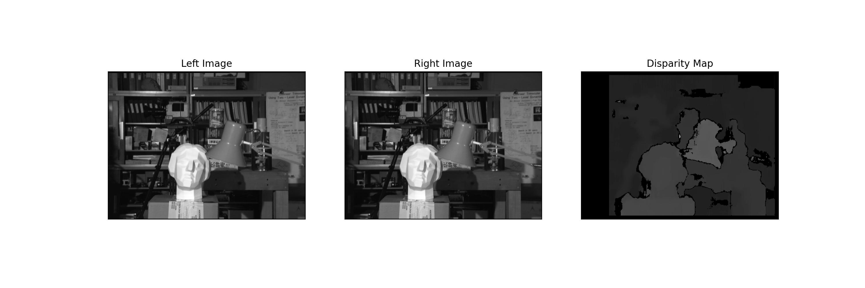
This code computes a Disparity Map from a pair of rectified stereo images using OpenCV's StereoBM block matching algorithm. Note: This requires a sample stereo pair. You can find standard pairs like 'tsukuba' from the Middlebury Stereo Vision dataset.
# Disparity Map Computation

import cv2
import numpy as np
from matplotlib import pyplot as plt

# NOTE: This example requires a rectified stereo image pair.
# Download a standard pair like 'tsukuba' from the Middlebury dataset
# and place 'tsukuba_l.png' and 'tsukuba_r.png' in your directory.
# For demonstration, we'll create a synthetic pair if files are not found.

try:
    imgL = cv2.imread('tsukuba_l.png', cv2.IMREAD_GRAYSCALE)
    imgR = cv2.imread('tsukuba_r.png', cv2.IMREAD_GRAYSCALE)
    if imgL is None or imgR is None: raise FileNotFoundError
except FileNotFoundError:
    print("Tsukuba images not found. Creating a synthetic stereo pair.")
    # Create a simple scene with objects at different depths
    imgL = np.full((300, 400), 200, dtype=np.uint8)
    imgR = imgL.copy()
    # Near object (large disparity)
    cv2.rectangle(imgL, (100, 100), (150, 150), 100, -1)
    cv2.rectangle(imgR, (100 - 20, 100), (150 - 20, 150), 100, -1)
    # Far object (small disparity)
    cv2.circle(imgL, (250, 150), 30, 50, -1)
    cv2.circle(imgR, (250 - 5, 150), 30, 50, -1)

# 1. Initialize Stereo Block Matcher
# numDisparities must be divisible by 16
stereo = cv2.StereoBM_create(numDisparities=16*3, blockSize=15)

# 2. Compute disparity map
disparity = stereo.compute(imgL, imgR)

# 3. Visualize results
plt.figure(figsize=(12, 6))
plt.subplot(1, 3, 1)
plt.imshow(imgL, 'gray')
plt.title('Left Image')
plt.xticks([]), plt.yticks([])

plt.subplot(1, 3, 2)
plt.imshow(imgR, 'gray')
plt.title('Right Image')
plt.xticks([]), plt.yticks([])

plt.subplot(1, 3, 3)
# Normalize the disparity map for visualization
disparity_visual = cv2.normalize(disparity, None, alpha=0, beta=255, norm_type=cv2.NORM_MINMAX, dtype=cv2.CV_8U)
plt.imshow(disparity_visual, 'gray')
plt.title('Disparity Map')
plt.xticks([]), plt.yticks([])

plt.suptitle("Stereo Vision - Disparity Calculation", fontsize=16)
plt.show()

# In the disparity map, brighter pixels correspond to larger disparity (closer objects).
Result: