Naive GEMM의 memory bottleneck부터 tiled reuse, Tensor Core pipeline, shape별 scheduling과 library 추상화까지
Topics
Abstract
GEMM(General Matrix Multiplication)은 두 행렬을 곱한 뒤 필요하면 기존 행렬을 더하는 연산이다. 딥러닝에서 자주 만나는 Linear layer, attention projection, MLP의 주된 계산이 모두 여기에 해당한다. 딥러닝 workload의 성능을 들여다보려면 GEMM이 어디서 빨라지고 어디서 느려지는지부터 짚어야 한다.
GEMM을 최적화할 때 먼저 볼 것은 multiply-add가 아니라 data movement다. Naive kernel은 output 하나를 thread 하나에 맡긴다. 이때 여러 thread가 같은 A와 B 원소를 global memory에서 반복해서 가져온다. Tiled kernel은 이런 중복 이동을 shared memory와 register의 재사용으로 바꾼다. Arithmetic intensity가 높아지면서 병목도 HBM bandwidth에서 on-chip bandwidth, instruction throughput, scheduling 쪽으로 옮겨 간다.
이 글에서는 먼저 GEMM의 수학적 정의와 naive 구현의 traffic을 살펴본다. 그 위에 shared-memory tiling, register blocking, Tensor Core pipeline을 차례로 쌓아 본다. 이후 shape-aware scheduling과 fusion 같은 고급 기법까지 범위를 넓힌다. cuBLAS, cuBLASLt, CUTLASS, CuTe의 위치는 마지막에 다룬다.
본문의 API와 아키텍처 설명은 2026년 8월, CUDA 13.3과 CUTLASS 4.6.1 공식 문서를 기준으로 확인했다. 지원 dtype, epilogue, scheduler와 instruction path는 toolkit과 GPU 세대에 따라 달라지므로 실제 적용 전에는 배포 환경의 문서와 API query를 다시 확인해야 한다.
1. GEMM의 정의
일반적인 GEMM은 다음 식을 계산한다.
$$ D=\alpha\,\operatorname{op}(A)\operatorname{op}(B)+\beta C $$
op는 matrix를 그대로 쓰거나 transpose하는 연산을 가리킨다. Transpose가 없는 경우 shape은
$$ A\in\mathbb{R}^{M\times K},\qquad B\in\mathbb{R}^{K\times N},\qquad C,D\in\mathbb{R}^{M\times N} $$
이다. Output 원소 하나는
$$ D_{ij}=\alpha\sum_{k=0}^{K-1}A_{ik}B_{kj}+\beta C_{ij} $$
로 계산한다. $M\times N$개의 dot product가 있고 각 dot product의 길이는 $K$다. Multiply와 add를 각각 1 FLOP로 세면 주된 matrix product의 연산량은 약
$$ 2MNK\quad\text{FLOPs} $$
이다. Alpha와 beta를 적용하는 연산은 이 근사에서 제외한다.
여기서 눈여겨볼 성질은 reuse다. $A_{ik}$ 하나는 같은 row의 $N$개 output에 쓰인다. $B_{kj}$ 하나는 같은 column의 $M$개 output에 쓰인다. 입력을 한 번만 읽고 이 reuse를 모두 활용한다면 행렬이 커질수록 byte당 계산량도 늘어난다.
물론 수식에 reuse가 보인다고 해서 kernel이 알아서 활용해 주지는 않는다. GPU에서 GEMM을 빠르게 만들려면 이 값을 memory hierarchy의 어느 단계에 둘지, 또 어떤 thread들이 나눠 쓸지를 정해야 한다.
2. Naive GEMM의 병목
가장 직접적인 병렬화는 output 원소 하나를 CUDA thread 하나에 맡기는 것이다. 아래 예제는 $D=AB$, 즉 $\alpha=1$, $\beta=0$, transpose 없음으로 제한하며 A, B, D가 row-major contiguous buffer라고 가정한다.
__global__ void naive_gemm(
    const float* A,
    const float* B,
    float* D,
    int M,
    int N,
    int K)
{
    int row = blockIdx.y * blockDim.y + threadIdx.y;
    int col = blockIdx.x * blockDim.x + threadIdx.x;

    if (row >= M || col >= N) {
        return;
    }

    float acc = 0.0f;
    for (int k = 0; k < K; ++k) {
        acc += A[row * K + k] * B[k * N + col];
    }
    D[row * N + col] = acc;
}
이 kernel은 정답을 내고 output parallelism도 충분히 드러낸다. 겉보기에는 별문제가 없어 보인다. 하지만 각 thread가 자신의 dot product를 따로 계산한다.
입력 재사용의 부재
Output 하나를 계산할 때 A에서 $K$개, B에서 $K$개를 읽는다. $MN$개의 output을 각각 따로 계산한다고 보면 logical input read는 모두
$$ 2MNK\quad\text{elements} $$
다. Input element 크기를 $b$ bytes, output element 크기를 $b_D$ bytes라 두면 traffic은 단순하게
$$ \text{bytes}_{\text{naive}} \approx 2bMNK+b_DMN $$
이고 arithmetic intensity는
$$ I_{\text{naive}} \approx \frac{2MNK}{2bMNK+b_DMN} \xrightarrow[K\to\infty]{} \frac{1}{b} $$
로 계산된다. 이 모델에서는 FP32 input이 약 0.25 FLOP/byte, FP16/BF16 input이 약 0.5 FLOP/byte에 그친다.
이 수치가 그대로 실제 DRAM traffic이 되는 것은 아니다. 같은 warp의 thread는 A 원소를 broadcast 받는다. B의 연속된 원소는 coalesced access가 된다. L1/L2 cache도 중복 요청 일부를 받아낸다. 위 계산에서 봐야 할 부분은 따로 있다. Output마다 독립적인 load instruction을 발행하면 kernel이 직접 관리하는 reuse가 생기지 않는다.
실제 HBM traffic은 cache hit와 transaction 형태에 따라 이 계산보다 작다. 다만 working set이 cache보다 크거나 여러 CTA가 cache capacity를 놓고 경쟁하면 같은 A/B tile이 L2와 HBM에서 반복해서 올라온다. “naive GEMM은 언제나 DRAM bandwidth peak에 닿는다”라고 단정할 수는 없다. 그래도 병목이 생기는 지점은 분명하다.
Naive GEMM은 수학적으로 가능한 A/B reuse를 kernel이 소유하지 않는다. 큰 problem에서는 global-memory load가 반복되고 arithmetic unit에 operand를 공급하는 경계가 병목이 되기 쉽다.
위 mapping은 row-major다. 한 warp가 같은 output row에서 연속된 column을 처리하면 B access는 coalesced된다. 같은 k의 A는 warp lane들이 한 주소를 함께 읽는다. Hardware broadcast 덕분에 transaction 수는 줄어든다. 다만 cache sector에서 실제로 쓰는 word는 적기도 하다. 다음 k에 필요한 cache line이 그때까지 남으리라는 보장도 없다. 여기에 다른 output row와 CTA가 같은 B tile을 다시 읽는 문제까지 더해진다. NVIDIA의 CUDA C++ Best Practices Guide에서도 shared memory를 써서 이 중복 transfer를 없애는 matrix multiplication 예제를 소개한다.
GEMM의 Arithmetic Intensity
A와 B를 각각 한 번만 읽고 D를 한 번 쓴다고 가정하면 $\beta=0$일 때 전체 연산의 이상적인 traffic은 대략
$$ b(MK+KN)+b_DMN $$
이다. $\beta\ne0$이면 C를 읽는 $b_CMN$ bytes가 더 든다. $M$, $N$, $K$가 함께 커질 때 FLOP은 cubic하게 늘고 input과 output element 수는 quadratic하게 늘어난다. GEMM은 원래 높은 arithmetic intensity를 만들 수 있는 연산이다. Naive mapping에서는 이 장점을 살리지 못한다.
Roofline 관점에서는
$$ P_{\text{attainable}} \leq \min\left(P_{\text{compute peak}},\ I\cdot B_{\text{memory}}\right) $$
이다. Naive implementation처럼 $I$가 낮으면 memory roof가 먼저 성능을 제한한다. 이제 줄여야 할 것은 FLOP이 아니다. 같은 FLOP을 처리하는 데 필요한 global-memory byte를 줄여 $I$를 높여야 한다.
3. Tiled GEMM과 데이터 재사용
Tiling에서는 가까운 output들을 한 CTA가 함께 계산한다. 필요한 A와 B 조각은 shared memory에 한 번만 올린다.
HBM / global memory
  A tile, B tile을 cooperative load
          ↓
Shared memory
  block의 여러 thread가 같은 tile을 재사용
          ↓
Registers
  각 thread가 output partial sum을 누적
          ↓
HBM / global memory
  완성된 output을 한 번 store
단순화한 square-tile kernel은 다음과 같다.
template <int TILE>
__global__ void tiled_gemm(
    const float* A,
    const float* B,
    float* D,
    int M,
    int N,
    int K)
{
    __shared__ float As[TILE][TILE];
    __shared__ float Bs[TILE][TILE];

    int tx = threadIdx.x;
    int ty = threadIdx.y;
    int row = blockIdx.y * TILE + ty;
    int col = blockIdx.x * TILE + tx;
    float acc = 0.0f;

    for (int k0 = 0; k0 < K; k0 += TILE) {
        As[ty][tx] = (row < M && k0 + tx < K)
            ? A[row * K + k0 + tx] : 0.0f;
        Bs[ty][tx] = (k0 + ty < K && col < N)
            ? B[(k0 + ty) * N + col] : 0.0f;

        __syncthreads();
        for (int k = 0; k < TILE; ++k) {
            acc += As[ty][k] * Bs[k][tx];
        }
        __syncthreads();
    }

    if (row < M && col < N) {
        D[row * N + col] = acc;
    }
}
첫 barrier를 지나야 tile 계산이 시작된다. 두 번째 barrier는 현재 계산이 끝나기 전에 다음 K tile이 shared-memory buffer를 덮지 못하게 막는다. Production kernel에서는 thread 하나가 여러 element를 맡아 더 큰 tile을 cooperative하게 load한다. 여기에 asynchronous pipeline과 register tile을 더한다.
Global-memory Traffic 감소
CTA 하나가 $B_M\times B_N$ output tile을 계산하고 K dimension을 $B_K$씩 순회한다고 하자. 한 K tile에서 필요한 input과 연산량은
$$ \begin{aligned} \text{A tile} &: B_MB_K,\\ \text{B tile} &: B_KB_N,\\ \text{compute} &: 2B_MB_NB_K\ \text{FLOPs}. \end{aligned} $$
A 원소 하나는 CTA 안에서 $B_N$개의 output에, B 원소 하나는 $B_M$개의 output에 재사용된다. Input을 HBM에서 한 번씩만 읽는다고 가정하면 input 기준 arithmetic intensity는
$$ I_{\text{tile,input}} \approx \frac{2B_MB_NB_K} {b(B_MB_K+B_KB_N)} = \frac{2B_MB_N}{b(B_M+B_N)}. $$
정사각형 tile $B_M=B_N=T$에서는
$$ I_{\text{tile,input}}\approx\frac{T}{b} $$
가 된다.
| CTA output tile | FP16/BF16 input ($b=2$) | FP32 input ($b=4$) |
|---|---|---|
| $64\times64$ | 약 32 FLOP/byte | 약 16 FLOP/byte |
| $128\times128$ | 약 64 FLOP/byte | 약 32 FLOP/byte |
같은 dtype에서 tile edge를 두 배로 키우면 이 단순 모델의 input reuse도 두 배로 늘어난다. Naive mapping에서는 cache에 맡겼던 재사용을 이제 CTA가 직접 관리한다. Cooperative load를 연속 주소에 맞추면 global access도 coalesced된다.
On-chip 병목
큰 tile이 언제나 빠른 것은 아니다. Tile을 키우면 다음 비용이 함께 증가한다.
- shared-memory capacity와 bandwidth
- thread별 accumulator register와 register pressure
- block barrier와 pipeline state
- problem boundary의 빈 lane과 tail waste
- CTA당 자원 사용 증가로 인한 residency 감소
위 식은 input traffic만 계산했다. D store, $\beta C$의 read, alignment와 padding, CTA 사이의 중복 load는 빠져 있다. K가 짧을 때는 output과 epilogue traffic의 비중이 커진다. M이나 N이 작다면 tile 수가 부족해 GPU 전체를 채우지 못하기도 한다.
Tiling은 “memory-bound를 완전히 해결하는 기법”이 아니다. HBM에서 shared memory로 같은 값을 반복해서 가져오던 병목을 줄였을 뿐이다. 그다음에는 shared-memory access, register reuse, compute instruction과 synchronization 가운데 무엇이 비싼지가 드러난다.
4. Hierarchical Tiling과 Tensor Core Pipeline
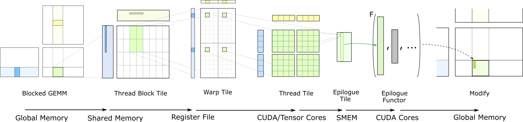
고성능 GEMM을 구현하려면 CTA tile 하나만으로는 부족하다. Output과 K reduction을 CUDA execution hierarchy와 memory hierarchy에 맞춰 한 번 더 나눈다.
Device GEMM
  ↓
CTA tile: global memory → shared memory, grid scheduling
  ↓
Warp / warp-group tile: shared-memory tile 분할
  ↓
MMA instruction tile: Tensor Core 또는 CUDA Core 연산
  ↓
Register / architecture-specific state: operand와 accumulator 재사용
Register blocking
Shared-memory tiling으로 HBM traffic을 줄이고 나면 shared-memory bandwidth가 다음 한계로 나타나기도 한다. Thread나 warp가 output scalar 하나 대신 작은 output tile을 맡는다고 해 보자. Shared memory에서 가져온 A fragment 하나를 여러 column accumulator에 쓴다. B fragment 하나도 여러 row accumulator가 나눠 쓴다.
Register blocking을 적용하면 shared-memory load당 FMA 수가 늘어난다. Partial sum도 mainloop 동안 register 가까이에 둔다. 대신 accumulator가 많아지는 만큼 register pressure가 커진다. Resident warp 수는 줄어들기도 한다. Register 수를 억지로 제한하다 local-memory spill이 생기면 앞에서 줄인 traffic이 다시 늘어난다.
Tensor Core Pipeline
Tensor Core instruction은 작은 matrix tile에
$$ D_{\text{frag}}\leftarrow A_{\text{frag}}B_{\text{frag}}+D_{\text{frag}} $$
를 수행한다. 하지만 이 instruction만으로 GEMM kernel이 완성되지는 않는다. Global-memory load, shared-memory layout, synchronization, tail handling, epilogue와 output store가 모두 필요하다. Tensor Core의 peak throughput이 높을수록 operand를 제때 공급할 tiling과 pipeline도 중요해진다.
Operand path는 architecture마다 다르다.
- Volta부터 Ampere까지 널리 사용된 warp-level MMA에서는 shared-memory operand를 thread별 register fragment로 옮기고 accumulator도 register에 둔다.
- Hopper WGMMA는 B를 shared-memory descriptor로 참조한다. 구성에 따라 A는 shared memory 또는 register에서 공급하고 accumulator는 register에 둔다. PTX ISA — WGMMA
- **Blackwell SM100
tcgen05.mma**는 accumulator를 Tensor Memory(TMEM)에 저장한다. A는 shared memory 또는 TMEM, B는 shared memory에서 공급할 수 있다. NVIDIA CUTLASS — tcgen05 MMA Programming Guide
그래서 모든 세대를 “thread register fragment” 하나로 묶어 설명하기는 어렵다.
Load–Compute Overlap
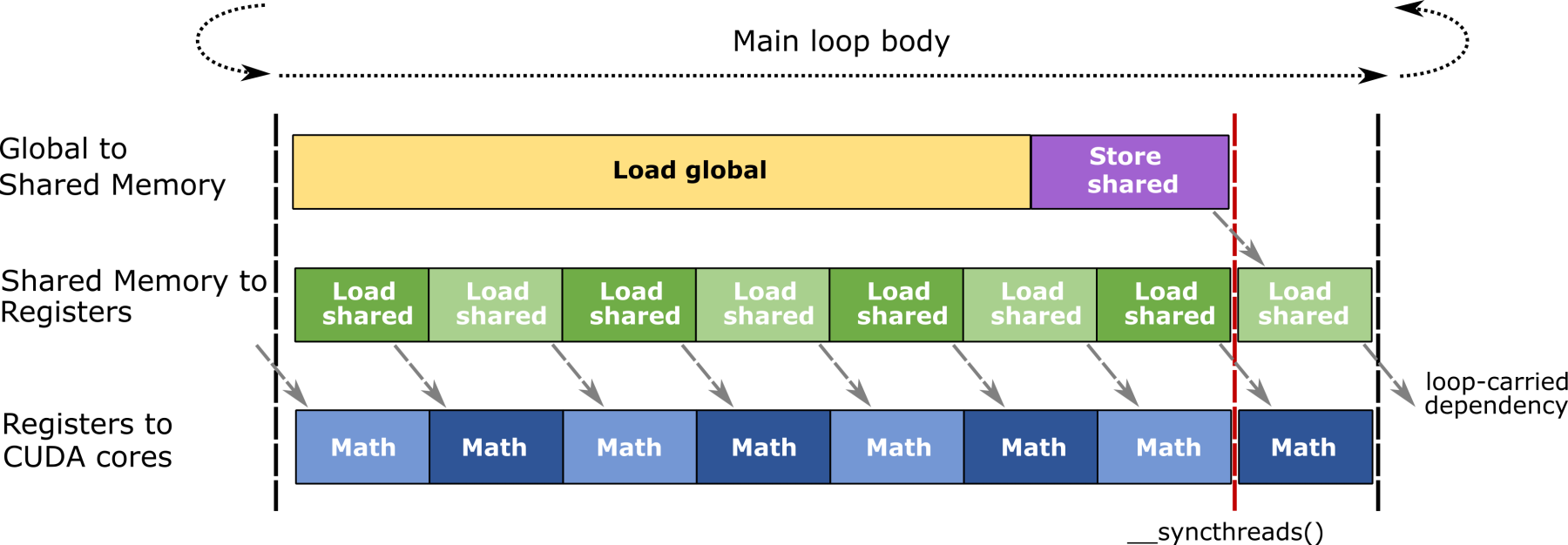
Tiling이 transfer byte를 줄이는 방법이라면, software pipelining은 아직 남은 transfer latency를 compute 뒤에 숨기는 방법이다.
load tile 0
wait tile 0

compute tile 0  ||  load tile 1
compute tile 1  ||  load tile 2
compute tile 2  ||  load tile 3
Double buffering과 multi-stage pipeline은 다음 tile을 미리 가져온다. 그만큼 shared-memory 사용량과 pipeline state는 늘어난다. Pipeline이 지나치게 깊으면 occupancy가 낮아진다. Short-K에서는 setup cost만 늘어난다. Ampere의 asynchronous copy, Hopper 이후의 TMA, 세대별 MMA와 barrier는 구현 방식은 달라도 load와 compute를 겹치는 데 쓰인다.
Epilogue
Mainloop가 끝나면 accumulator를 output layout에 맞춰 global memory에 저장한다. 지원하는 조합이라면 epilogue에서 alpha, beta, bias, activation, clamp와 dtype conversion을 같은 단계에 처리한다.
지원되는 epilogue를 쓰면 GEMM result를 저장한 뒤 별도 kernel이 다시 읽어야 하는 intermediate round trip이 사라진다. Irregular indexing이나 무거운 transform까지 억지로 넣어 mainloop throughput이 떨어진다면 이야기가 다르다. 이때는 tuned GEMM 뒤에 작은 kernel을 따로 실행하는 쪽이 더 빠르기도 하다.
5. Tiling 이후의 병목
모든 GEMM shape에 잘 맞는 tile과 pipeline은 없다. Large square GEMM에는 output tile이 충분하고 steady-state mainloop도 길다. Small-M, short-K, tail-heavy problem은 전혀 다른 비용에 막힌다.
| 관찰된 problem | 실제 병목 | 검토할 기법 | 추가 비용 |
|---|---|---|---|
| 큰 M/N/K와 규칙적인 shape | compute throughput, operand feed | 큰 CTA·warp tile, 깊은 pipeline, Tensor Core | register/shared-memory pressure |
| M/N이 작고 K가 김 | output tile과 execution wave 부족 | Split-K, Stream-K 계열 | partial reduction, workspace/atomic, 달라진 덧셈 순서 |
| Tile 경계에 remainder가 큼 | inactive lane과 tail waste | 더 작은 tile, predication, residue 전용 kernel | kernel 후보와 dispatch 증가 |
| 같은 shape의 small GEMM 다수 | launch와 scheduling 비중 | strided batched GEMM | batch 내부 shape·layout 제약 |
| 서로 다른 small GEMM 다수 | problem별 tail과 load imbalance | grouped persistent GEMM | metadata 탐색과 ordering |
| $M\approx1$인 batch-1 linear | 부족한 parallelism과 weight traffic | GEMV/small-M kernel, batching, weight prepacking | 전용 layout, batching latency |
| Quantized input 또는 post-op | decode·intermediate traffic | mainloop prologue, fused epilogue | register pressure, 지원 조합 제한 |
Split-K는 한 output tile의 K range를 여러 worker가 나눈다.
$$ P^{(s)}_{ij}=\sum_{k\in K_s}A_{ik}B_{kj},\qquad P_{ij}=\sum_sP^{(s)}_{ij} $$
K 방향의 병렬성은 늘어난다. 대신 partial sum을 저장하고 다시 합쳐야 한다. 기존 M/N tile만으로 GPU를 충분히 채우는 상황이라면 reduction 비용 때문에 오히려 느려진다. Stream-K 계열 역시 work를 더 고르게 나누는 대가로 scheduler와 fix-up 비용을 치른다.
Small-M GEMM에서는 M 방향 tile 수가 줄어든다. 같은 weight B를 여러 output row에 재사용할 기회도 적어진다. 이때는 큰 GEMM용 tile의 nominal TFLOPS만 봐서는 안 된다. 먼저 볼 값은 absolute latency, weight byte, active CTA 수다. 여러 request를 batching하면 B reuse와 parallelism이 늘지만 그만큼 대기 latency가 생긴다.
Tile tail에서는 경계에 남는 크기를 살펴야 한다. $M=130$인데 CTA tile의 M 크기가 64라면 세 번째 tile에서 실제로 쓰는 row는 2개뿐이다. 이런 경우에는 큰 tile의 peak throughput보다 boundary waste가 성능을 더 크게 좌우한다.
Precision을 기록할 때는 input, compute/accumulator, output dtype을 나눠야 한다. BF16 input, FP32 accumulator, BF16 output이 한 조합이다. FP8과 block-scaled format이라면 scale dtype과 granularity도 적어야 한다. Split-K, scheduler와 epilogue가 reduction order나 rounding boundary를 바꾸면 같은 GEMM 식에서도 bitwise result가 달라질 수 있다.
6. 추상화 계층
지금까지는 kernel이 최적화되는 과정을 아래에서 위로 따라왔다. 실제 제품을 구현할 때는 반대로 접근한다. 요구사항을 표현할 수 있는 가장 높은 계층에서 시작하면 된다.
Mathematical operation
  GEMM semantics and shapes
        ↓
Library / API
  cuBLAS → cuBLASLt
        ↓
Kernel construction
  CUTLASS device operators → CuTe components
        ↓
Custom implementation
  CUDA C++ / architecture-specific instructions
        ↓
Hardware
  scheduler, SM, Tensor Core, register, shared memory, HBM
| 필요한 것 | 첫 후보 | 한 단계 아래로 내려갈 조건 |
|---|---|---|
| 표준 dense GEMM | cuBLAS | layout, epilogue, workspace, algorithm 후보를 더 제어해야 함 |
| 유연한 layout·compute type·epilogue | cuBLASLt | API가 필요한 조합이나 dataflow를 표현하지 못함 |
| Custom mainloop·quantized decode·scheduler | CUTLASS device operator / CuTe component | 제공된 구성 요소로도 요구사항을 표현하거나 유지하기 어려움 |
| 완전히 특수한 dataflow | Custom CUDA kernel | 측정된 이득이 구현·검증·이식 비용보다 큼 |
cuBLASLt는 cuBLAS의 상위 버전이 아니다. Layout, algorithm, heuristic과 epilogue를 더 유연하게 기술하는 별도 API다. CUTLASS나 CuTe로 작성했다고 해서 library보다 빠른 것도 아니다.
원리를 이해할 때는 naive kernel에서 시작해 위로 올라간다. 제품 구현은 cuBLAS에서 시작해 필요한 만큼만 아래로 내려가면 된다.
Shape Manifest
추상화 계층을 고르기 전에 production path의 shape를 수집한다.
name, M, N, K, batch/group, transA, transB,
A/B/C/D layout and dtype, compute type,
alpha, beta, epilogue, alignment,
workspace limit, frequency or probability
평균 shape 하나만 보면 tail, small-M, short-K와 heterogeneous group을 놓치기 쉽다. 표준 연산에서는 cuBLAS를 baseline으로 잡고 같은 조건의 cuBLASLt heuristic 후보와 비교한다. API로 요구사항을 표현할 수 없거나 중요한 shape에서 같은 병목이 반복될 때 CUTLASS 또는 custom kernel을 후보에 넣는다.
측정할 때는 다음을 함께 남긴다.
- Small GEMM은 TFLOPS보다 median·tail absolute latency를 우선한다.
- Large GEMM은 latency와 achieved FLOP/s를 함께 보고 Nsight Compute에서 SM/Tensor Core utilization, DRAM·L2 traffic을 확인한다.
- Custom tile은 register 수, spill, shared-memory 사용량, occupancy와 tail utilization을 기록한다.
- Fused epilogue나 quantized decode는 pure GEMM이 아니라 호출 전후의 end-to-end interval을 잰다.
- Allocation과 copy는 측정 구간 밖으로 옮긴다. Production이 cache-hot이 아니라면 여러 buffer를 rotation한다. NVIDIA CUTLASS — GEMM Performance Measurement Methodology
Input, compute, output dtype에 맞는 reference와 tolerance도 정해 둔다. Byte-exact reproducibility가 필요하다면 toolkit, GPU architecture, algorithm과 workspace configuration을 함께 고정해야 한다. 그 정도의 재현성이 필요하지 않다면 application에 의미 있는 error bound를 사용한다. NVIDIA cuBLAS — Results Reproducibility
GEMM 최적화 기준
Naive GEMM이 느린 이유를 thread 수에서 찾으면 안 된다. 각 output을 계산할 때 같은 operand를 계속 옮기는 것이 문제다. Shared-memory tiling은 A와 B를 CTA 안에서 재사용해 global-memory byte를 줄인다. Register blocking은 같은 방식을 warp와 thread 수준에 적용한다. 이렇게 dataflow를 정리한 다음에야 Tensor Core와 software pipeline으로 compute throughput을 높이고 latency를 숨긴다.
여기까지 오면 shape가 답을 바꾼다. Small-M, short-K, tail, batching, quantization과 epilogue마다 병목이 다르고 잘 맞는 scheduler도 달라진다. cuBLAS, cuBLASLt, CUTLASS, CuTe, custom CUDA는 이런 선택을 서로 다른 높이에서 다루는 도구다. 무조건 가장 낮은 계층으로 내려갈 필요는 없다. 실제 병목을 해결하는 데 필요한 만큼만 드러내는 계층을 고르면 된다.
References
- NVIDIA, cuBLAS 13.3 Documentation: https://docs.nvidia.com/cuda/cublas/
- NVIDIA, cuBLASLt API: https://docs.nvidia.com/cuda/cublas/#using-the-cublaslt-api
- NVIDIA, CUDA C++ Best Practices Guide — Shared Memory in Matrix Multiplication: https://docs.nvidia.com/cuda/cuda-c-best-practices-guide/#shared-memory-in-matrix-multiplication-c-ab
- NVIDIA, CUTLASS 4.6.1 Documentation: https://docs.nvidia.com/cutlass/latest/overview.html
- NVIDIA, Efficient GEMM in CUDA: https://docs.nvidia.com/cutlass/latest/media/docs/cpp/efficient_gemm.html
- NVIDIA, CUTLASS GEMM API: https://docs.nvidia.com/cutlass/latest/media/docs/cpp/gemm_api.html
- NVIDIA, GEMM Performance Measurement Methodology Guidelines: https://docs.nvidia.com/cutlass/latest/media/docs/cpp/gemm_performance_measurement_methodology_guidelines.html
- NVIDIA, PTX ISA — WGMMA: https://docs.nvidia.com/cuda/parallel-thread-execution/#asynchronous-warpgroup-level-matrix-multiply-accumulate-instructions-wgmma
- NVIDIA, tcgen05 MMA Programming Guide: https://docs.nvidia.com/cutlass/latest/media/docs/pythonDSL/mma_docs/tcgen05_programming.html
- NVIDIA, Grouped Kernel Schedulers: https://docs.nvidia.com/cutlass/latest/media/docs/cpp/grouped_scheduler.html