From sparse quadratic solvers in quad remeshing to deep learning optimizers
Topics
Background: Quad Remeshing & DiT
My research work this year has centered on two projects.
One is training a high-quality image-conditioned 3D generative model based on a DiT. The other is developing a high-quality quad remesher for VARCO3D. Beyond their shared focus on 3D, graphics algorithms and generative model training differ considerably in both their implementation and the literature they draw on.
To briefly describe the remeshing problem: I first compute a cross field on the input triangle mesh to specify how the quads should align, then solve for a globally consistent integer coordinate system that follows this field as closely as possible. This can be viewed as a Poisson-type PDE that brings the gradients of the unknown coordinates as close as possible to the prescribed directions. Integer constraints on how the mesh surface connects, however, turn it into a mixed-integer quadratic (MIQ) optimization problem.
I covered the full pipeline in my earlier post, Comprehensive Analysis of Quad Remeshing.
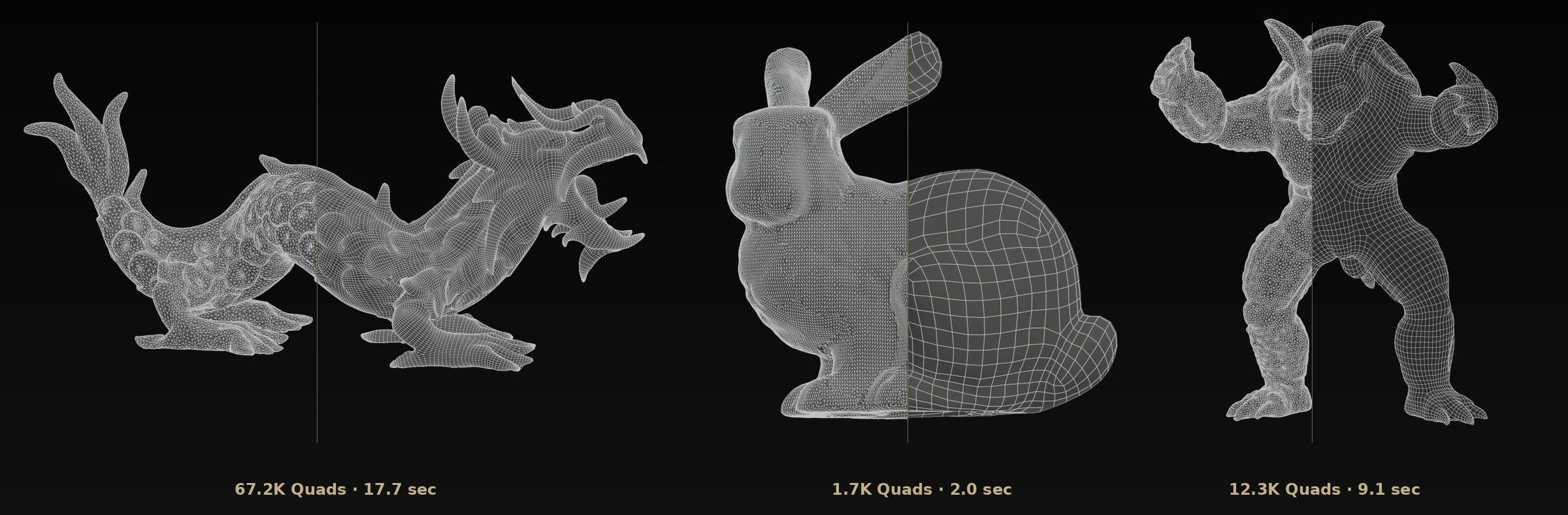
MIQ problems are NP-hard in general. Rather than search over every integer assignment, my implementation accelerates a relax-and-fix approach on the GPU: first solve the continuous relaxation, choose some variables to round and fix, then minimize the energy over the remaining variables. This is an approximate method that alternates between integer decisions and continuous optimization.
While accelerating this computation in CUDA, I found that parallelizing the operations was only part of the problem. The numerical method—and how many iterations it needed to reach the target accuracy—mattered just as much. After comparing several configurations, I settled on 2×2 block-Jacobi PCG (Preconditioned Conjugate Gradient), which was the fastest in practice, as the default solver.
Meanwhile, in my DiT training experiments for 3D generation, I was trying the Muon optimizer on matrix-valued parameters. Muon required some extra care: non-matrix parameters still needed an optimizer such as AdamW, and compared with the familiar AdamW setup, improving update speed required optimizing the kernels myself.
Muon's update rule reminded me of the PCG solver I was using in the remesher. Neither PCG nor Muon uses the gradient directly. Both try to stabilize and accelerate updates through a kind of coordinate transformation.
Could numerical preconditioners and deep learning optimizers be serving fundamentally similar roles? How would they behave on the same quadratic objective? Could Muon or Adam work for quad remeshing?
1. Quadratic Objectives & Conjugate Gradient
Let us start with a simple quadratic objective. Assuming that $H$ is symmetric positive definite (SPD), the objective, its gradient, and the optimality condition are
$$ f(x)=\frac12x^\top Hx-b^\top x $$ $$ g(x)=Hx-b,\qquad Hx^*=b $$
Gradient descent (GD) moves against the current gradient:
$$ x_{k+1}=x_k-\eta g_k $$
For a fixed Euclidean step length, this is the direction that decreases the first-order approximation of the objective the most. It becomes inefficient, however, when the curvature differs across axes.
For example, in
$$ f(x_1,x_2)=50x_1^2+\frac12x_2^2 $$
the curvature along $x_1$ is 100 times that along $x_2$. Reducing the step size enough to avoid divergence in the high-curvature direction makes convergence in the flatter direction extremely slow.
Even exact line search, which finds the optimal step length along the gradient at every iteration, does not resolve this problem. After a line search, the new gradient is orthogonal to the previous search direction, but later steps need not preserve the optimality already achieved along that direction. This produces the familiar zigzagging path through long, narrow elliptical contours. Its behavior is governed by the curvature imbalance, expressed by the condition number $\kappa(H)=\lambda_{\max}(H)/\lambda_{\min}(H)$.
H-Conjugacy: Preserving Earlier Progress
Conjugate Gradient (CG) requires its search directions to be orthogonal under an inner product defined by the objective's curvature $H$, rather than under the Euclidean inner product. This is called $H$-conjugacy:
$$ p_i^\top Hp_j=0\qquad(i\ne j) $$
If the current point $x$ has already been optimized along $p_i$, then $p_i^\top g(x)=0$. After moving in a new direction $p_j$, the gradient component along $p_i$ is
$$ p_i^\top g(x+\alpha p_j) = \underbrace{p_i^\top g(x)}_{0} + \alpha\underbrace{p_i^\top Hp_j}_{0} =0 $$
Moving in a new $H$-conjugate direction therefore preserves optimality along the directions we have already optimized. CG uses this property to expand its search space.
Define the residual as
$$ r_k=b-Hx_k=-g_k $$
Starting with the initial direction $p_0=r_0$, the algorithm needs only the following short recurrence:
$$ \begin{aligned} x_{k+1}&=x_k+\alpha_kp_k, & \alpha_k&=\frac{r_k^\top r_k}{p_k^\top Hp_k},\\ r_{k+1}&=r_k-\alpha_kHp_k,\\ p_{k+1}&=r_{k+1}+\beta_kp_k, & \beta_k&=\frac{r_{k+1}^\top r_{k+1}}{r_k^\top r_k}. \end{aligned} $$
For a fixed SPD quadratic in exact arithmetic, CG reaches the exact solution in at most as many iterations as there are variables. In floating-point arithmetic, rounding errors gradually erode orthogonality and conjugacy, so this theoretical finite-step convergence cannot be taken literally.
From an implementation perspective, CG's appeal is that it uses curvature information through a single sparse matrix-vector multiplication (SpMV), $Hp_k$, per iteration, without ever forming the inverse Hessian. This SpMV was also the main operation I was optimizing in CUDA.
Mixing the previous direction $p_k$ into the current direction may look like momentum in deep learning. The distinction is that ordinary momentum accumulates past gradients with a fixed coefficient, whereas CG recomputes $\beta_k$ at every step specifically to preserve conjugacy with the previous direction.
2. Preconditioning: The Geometry of a Norm
Even when CG chooses its search directions efficiently, an unfavorable Hessian eigenvalue distribution can still make convergence slow. Preconditioning transforms the coordinate system itself to address this.
Introduce an SPD matrix $M$ that approximates $H$, and change coordinates using
$$ x=M^{-1/2}y $$
The Hessian in the new coordinates becomes
$$ \widetilde H=M^{-1/2}HM^{-1/2} $$
Ideally, if $M=H$, then $\widetilde H=I$, giving equal curvature in every direction. The elongated elliptical geometry that hinders convergence becomes a spherical geometry that is much easier to optimize.
Computing $H^{-1}$ is too expensive in practice. The goal is therefore to find an $M$ that is inexpensive to apply while sufficiently reducing the curvature imbalance in $\widetilde H$. PCG applies CG to this transformed problem.
Another way to view preconditioning is as a change in the metric used to measure update size, from the Euclidean norm to the $M$-norm:
$$ \|\Delta x\|_M^2=\Delta x^\top M\Delta x $$
Minimizing a first-order approximation under the corresponding quadratic penalty gives
$$ \Delta x^* = \arg\min_{\Delta x} \left[ g^\top\Delta x+ \frac{1}{2\eta}\Delta x^\top M\Delta x \right] = -\eta M^{-1}g $$
The direction of steepest descent thus depends on more than the gradient at the current point. It also depends on the geometry in which we measure the step.
Standard PCG applies this transformation to the residual, computing $z_k=M^{-1}r_k$ and updating as follows:
$$ p_{k+1}=z_{k+1}+\beta_kp_k, \qquad \alpha_k=\frac{r_k^\top z_k}{p_k^\top Hp_k}, \qquad \beta_k=\frac{r_{k+1}^\top z_{k+1}}{r_k^\top z_k} $$
2×2 Block-Jacobi vs. Incomplete Cholesky (IC)
The remesher's 2×2 block-Jacobi preconditioner groups strongly coupled variables into pairs and extracts their Hessian submatrices. If $B_i$ denotes the indices of a selected pair, its diagonal block is
$$ H[B_i,B_i] = \begin{pmatrix} a_i&c_i\\ c_i&b_i \end{pmatrix} $$
Unlike scalar Jacobi, which uses only diagonal entries, this captures the cross term $c_i$ between the two variables. It ignores coupling outside the block, but each 2×2 block can be inverted completely independently, making it well suited to GPU parallelism.
Incomplete Cholesky (IC), by comparison, constructs a sparse approximate factorization $H\approx LL^\top$. By capturing coupling over a wider range of variables, it can substantially reduce the number of iterations needed to converge. Applying the preconditioner, $z_k=M^{-1}r_k$, however, requires two triangular solves (SpSV) per iteration:
$$ Ly=r,\qquad L^\top z=y $$
Triangular solves have inherent sequential dependencies: some variables cannot be solved until earlier results are available. The available parallelism also depends heavily on the matrix's sparsity pattern. NVIDIA Docs
Ultimately, total solve time is the product of the number of iterations needed to converge and the cost of each iteration. This tradeoff showed up clearly in the experiments below.
3. Adam and Muon
Deep learning optimizers also transform the gradient before using it, but they construct those transformations from different information than numerical preconditioners do.
Adam: Gradient-Based Diagonal Scaling
Adam maintains exponential moving averages (EMAs) of the gradient's first and second moments:
$$ m_t=\beta_1m_{t-1}+(1-\beta_1)g_t, \qquad v_t=\beta_2v_{t-1}+(1-\beta_2)g_t^{\odot2} $$
Using the bias-corrected estimates $\hat m_t$ and $\hat v_t$, its update is
$$ \Delta x_t = -\eta \frac{\hat m_t}{\sqrt{\hat v_t}+\epsilon} $$
Writing the denominator as a diagonal matrix $D_t$ gives
$$ \Delta x_t=-\eta D_t^{-1}\hat m_t $$
In this form, Adam looks like momentum with adaptive diagonal preconditioning.
Unlike Jacobi PCG, which uses the actual diagonal of the Hessian, Adam uses an average of squared gradients observed along its optimization trajectory. Averaging gradient magnitudes does not recover the objective's Hessian. In a noise-free, deterministic quadratic such as the one in these experiments, $g(x)=Hx-b$ is available exactly, so Adam's $v_t$ depends entirely on the path taken from the starting point.
Muon: Steepest Descent in the Spectral Norm
Muon operates on parameters that take the form of two-dimensional matrices. Let $B_t$ be the matrix obtained by combining momentum and Nesterov acceleration. An idealized Muon orthogonalizes this matrix by setting all positive singular values to 1—more precisely, by extracting the orthogonal factor of its polar decomposition:
$$ B_t=U_r\Sigma_rV_r^\top \quad\Longrightarrow\quad Q_t=U_rV_r^\top $$
Instead of performing an expensive SVD at every step, practical implementations approximate this transformation with a polynomial using Newton–Schulz iterations. They use only a few iterations and do not guarantee that the result matches the exact polar factor.
The geometry of this operation can also be understood as a change of norm. Setting momentum aside for a moment, let $G$ be the current gradient matrix. Consider minimizing the linearized loss subject to a bound on the spectral norm $\|\cdot\|_2$, the largest singular value of a matrix:
$$ \min_{\|\Delta W\|_2\leq\eta} \langle G,\Delta W\rangle \quad\Longrightarrow\quad \Delta W^*=-\eta U_rV_r^\top $$
Muon's orthogonalization thus finds a steepest-descent direction under the spectral norm.
For a linear layer $y=Wa$, the output change caused by a weight update satisfies
$$ \|\Delta W a\|_2 \leq \|\Delta W\|_2\|a\|_2 $$
The design treats the parameters as an operator mapping inputs to outputs, rather than as a flat vector, and controls the change in the output accordingly.
- This interpretation of optimizers as steepest descent under particular norms is also developed in work such as Old Optimizer, New Norm. arXiv
- Jeremy Bernstein's derivation of Muon
We can now see both the connection and the distinction between PCG and Muon. Both change the metric governing a step, but they act on different objects. PCG tries to flatten the eigenvalue spectrum of the objective's Hessian, while Muon flattens the singular-value spectrum of the update matrix itself.
The resemblance between the two was what prompted this post.
4. Experiments: Deep Learning Optimizers for Quad Remeshing
After working through the theory, I still wanted to know whether Muon or Adam could be useful in the MIQ solve for quad remeshing. I ran experiments to compare both their convergence behavior and their actual computational cost on hardware.
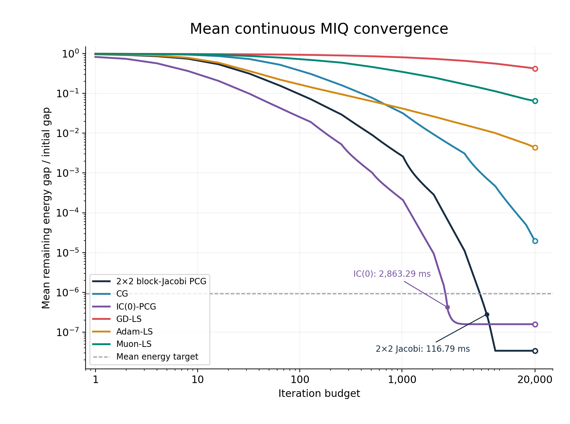
I compared six methods on matrices extracted from real remeshing problems: GD, CG, 2×2 block-Jacobi PCG, IC(0)-PCG, Adam, and Muon. To isolate quadratic solver performance, I held all other conditions fixed and measured only the MIQ energy minimization. The experiments ran on an NVIDIA B300 GPU, with FP64 used throughout.
Deep Learning Optimizers with Line Search
Running deep learning optimizers with fixed learning rates can make the comparison depend heavily on how well each learning rate has been tuned.
To compare the quality of the search directions they produce, I combined GD, Adam, and Muon with exact quadratic line search, denoting them GD-LS, Adam-LS, and Muon-LS in the experiments:
$$ x_{\mathrm{new}}=x+\alpha^* d, \qquad \alpha^*=-\frac{g^\top d}{d^\top Hd} $$
Adam retained its momentum estimates. Muon used momentum of 0.95, Nesterov acceleration, and five Newton–Schulz steps, with weight decay disabled. If a momentum-based direction was not a descent direction, I replaced it with the residual direction for that step and reset the momentum buffer.
- For idealized Muon without momentum, $Q=\operatorname{Polar}(G)$, the numerator in the line search becomes the nuclear norm $\|G\|_*$. The optimal step length is then $\alpha^* = \frac{\|G\|_*}{\langle Q,\mathcal H[Q]\rangle}$. Taking this optimal step still does not give the directions CG-style conjugacy.
Evaluation Criteria
I used two separate settings for a fair comparison:
- Continuous relaxation: Replay only the initial continuous optimization stage under the same conditions.
- Fixed integer assignment: Fix the final integer assignment selected by the default solver, initialize all free coordinates to zero, and solve the resulting single quadratic.
I measured convergence using the physical energy to compare how much each method reduced the actual remeshing objective. If $E_{\mathrm{ref}}$ is the energy reached by the default solver, I measured the iterations and time required to satisfy
$$ E\leq E_{\mathrm{ref}} +10^{-5}\max(|E_{\mathrm{ref}}|,1) $$
This energy includes only the least-squares terms, excluding the gauge terms added for numerical stability. The criterion therefore does not measure the error relative to the exact optimum or require an identical residual.
Although the theoretical discussion assumes SPD matrices, the extracted systems contain coordinates that are completely masked to zero, making the full matrices positive semidefinite (PSD). The experiments ran without issue on the active subspace with compatible right-hand sides.
5. Results
IC(0)-PCG vs. Block-Jacobi PCG
For the fixed-integer problems, the average iteration counts and execution times required to reach the target energy were:
| 2×2 block-Jacobi PCG | IC(0)-PCG |
|---|---|
| 142 iterations / 4.318 ms | 49 iterations / 103.946 ms |
As expected, IC(0) reduced the iteration count by roughly a factor of 3. Yet its actual GPU elapsed time was 24 times longer.
These timings already exclude the factorization cost of constructing the preconditioner. Kernel profiling showed that the two triangular solves per iteration, implemented with cuSPARSE SpSV, consumed most of the GPU execution time. Capturing more coupling information reduced the step count, but the sequential dependencies involved in applying that information prevented the solver from making good use of the GPU's parallel resources. The 2×2 block-Jacobi method needed more steps, but each was cheap and fully parallel, giving it a substantial advantage in total time.
- This result is specific to IC(0) with natural ordering and the current cuSPARSE implementation. Coloring or other reorderings could change the outcome.
Convergence Rates of GD, Adam, and Muon
The following table shows the fraction of runs that reached the target energy within a budget of 20,000 iterations. Failure here means the method did not converge within the budget, rather than that it diverged.
| Method | Continuous relaxation | Fixed integer assignment |
|---|---|---|
| CG | 79% | 100% |
| 2×2 block-Jacobi PCG | 100% | 100% |
| IC(0)-PCG | 100% | 100% |
| GD-LS | 0% | 53% |
| Adam-LS | 0% | 100% |
| Muon-LS | 0% | 21% |
On the easier fixed-integer problems, Adam-LS reached the target in all cases, but was 8.6–25.8 times slower than block-Jacobi. Muon-LS converged only for the smallest MIQ setting; in the other cases, it still had not reached the target after all 20,000 iterations.
| Continuous Relaxation | Fixed Integer Assignment |
|---|---|
 |
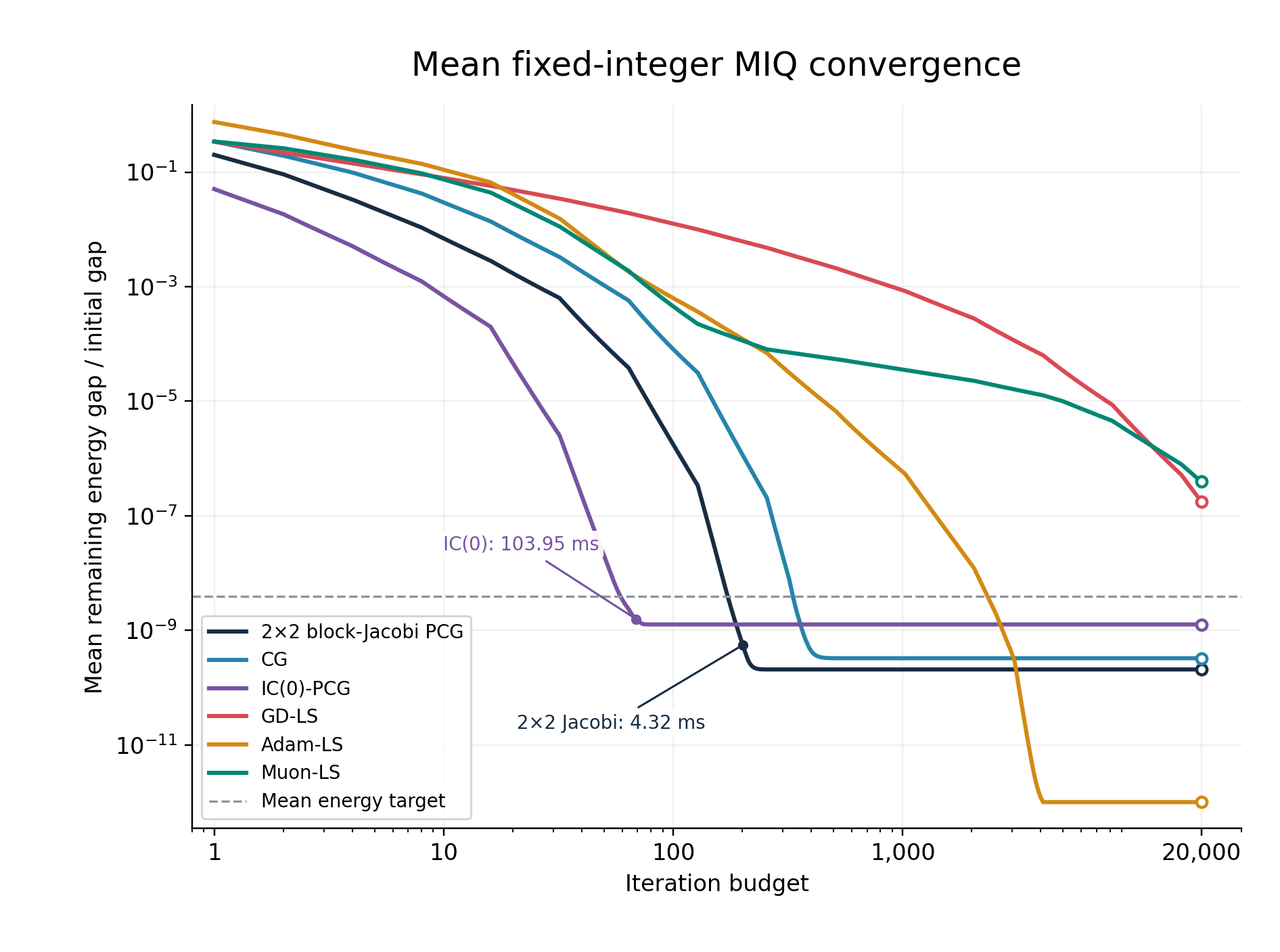 |
Muon's difficulty was not just the computational cost of running Newton–Schulz iterations at every step. It also needed far too many optimization iterations.
Deep learning typically involves substantial stochastic noise and no explicitly available Hessian. These sparse quadratic problems instead provide an exact Hessian and demand high-accuracy solutions. In this setting, equalizing the singular values of the update matrix could not replace PCG's conjugacy and curvature correction.
6. Reshaping for Muon
There was another detail to examine in these experiments. A DiT's linear layers have a natural two-dimensional structure defined by their input and output dimensions, whereas the remesher's variables form a one-dimensional vector. Applying Muon requires reshaping that vector into a matrix somehow.
Initially, I kept the original variable ordering and tried matrix widths of 1, 2, 8, 32, and 128, padding unused entries with zeros and restoring the original vector after each update.
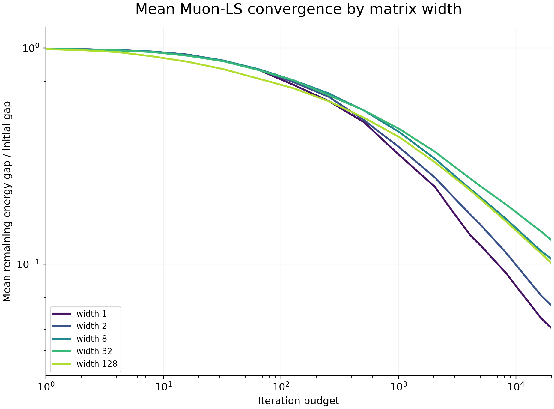
Increasing the width did not consistently improve convergence. In fact, width 1 sometimes reached a lower energy later in the solve.
- At width 1, the transformation normalizes the entire vector, so exact line search cancels out its scaling effect. Momentum and Nesterov acceleration are still present, however, so the trajectory differs from pure GD-LS. An idealized polar-LS method with momentum removed completely and width set to 1 is exactly equivalent to GD-LS.
Physical UV Pairs vs. the Hessian
What if, instead of splitting the vector arbitrarily, I built the matrix around the problem's geometric meaning?
The remeshing variables come from a two-dimensional coordinate map, $(u_i,v_i)$, at each vertex. By tracing the data indices, I recovered roughly 93–99% of the active variables as actual $(u_i,v_i)$ pairs belonging to the same vertex, arranged them in an $N\times 2$ matrix, and ran Muon again.
This physically meaningful UV pairing still performed no better than the original arbitrary width-2 arrangement.
While inspecting the Hessian entries to understand why, I found something interesting. In every $2\times 2$ diagonal Hessian block corresponding to a recovered physical $(u_i,v_i)$ pair, the cross terms were zero:
$$ H[\{u_i,v_i\},\{u_i,v_i\}] = \begin{pmatrix} a_i&0\\ 0&b_i \end{pmatrix} $$
There was no direct cross term between $u_i$ and $v_i$ at the same vertex. This does not mean that the U and V variable groups are entirely uncoupled; other coupling, such as that introduced by boundary conditions, may still exist.
Had I built a 2×2 block-Jacobi preconditioner around these physical UV pairs, it would have behaved exactly like scalar Jacobi because the cross terms vanish. The existing solver's 2×2 block-Jacobi routine, by contrast, greedily pairs variables with large off-diagonal entries $c_i$ in the actual Hessian, regardless of their physical meaning. Variables that form a physical pair were not the same variables that were strongly coupled numerically.
Muon's Gram Matrix
Even if those cross terms had been nonzero, the $2\times 2$ matrices used by block-Jacobi and width-2 Muon would still contain entirely different information.
For an $N\times 2$ gradient matrix $G$, consider the ideal polar transformation
$$ Q=G(G^\top G)^{-1/2} $$
The matrix whose inverse square root is taken here is the global Gram matrix
$$ G^\top G = \begin{pmatrix} \sum_i g_{u_i}^2 & \sum_i g_{u_i}g_{v_i}\\ \sum_i g_{u_i}g_{v_i} & \sum_i g_{v_i}^2 \end{pmatrix} $$
Block-Jacobi individually inverts the local curvature $H[B_i,B_i]$ for each pair of variables. Muon normalizes global correlations between axes, aggregating gradients over all vertices. Both may involve $2\times 2$ matrix operations, but what they correct is different.
Closing Thoughts
I am naturally drawn to algorithms that are mathematically elegant and rigorous. IC seemed promising because it captures more coupling between variables than block-Jacobi does. It did substantially reduce the iteration count. Once I accounted for the cost of applying that correction on the GPU, though, the simple 2×2 block-Jacobi method was much faster. My expectation about convergence was right, but it did not translate into the speedup I needed.
Muon followed a similar pattern. I initially thought of it as correcting a matrix imbalance in much the same way as block-Jacobi, then found that it was slow when I applied it. Had I stopped at the performance comparison, I would still not have understood why. Examining the different information carried by local Hessian blocks and the global Gram matrix, and the distinction between physical UV pairs and the strongly coupled pairs chosen by the solver, helped me understand how far the initial analogy could be trusted.
Over the past few months of developing a quad remesher and training 3D generative models, I have repeatedly found that turning a theoretically attractive idea into a practical performance improvement is a separate problem. Even a good hypothesis needs to be tested on real data and hardware. Convergence rates matter, but so does the price paid to achieve them. IC(0) can converge in fewer iterations yet run much more slowly on a GPU, and Muon may deliver worse results than the AdamW I was already using (billion-scale image-to-3D runs showed no qualitative gains and slower updates).
It has become much easier to implement ideas and run experiments. These days, I often find it more useful to try a candidate directly than to spend a long time debating it. I do not think this makes theoretical understanding less important. If anything, it makes it more important. A result that says “this is slow” does not tell me whether to discard the method, improve the implementation, or change how the variables are grouped. To make that decision, I still need to examine the mathematics, the data, and the code together. Here, that meant isolating the cost of triangular solves for IC, and looking separately at how Muon's matrices were assembled and what information its operations used. Those checks helped me decide what to try next with the GPU time I had.
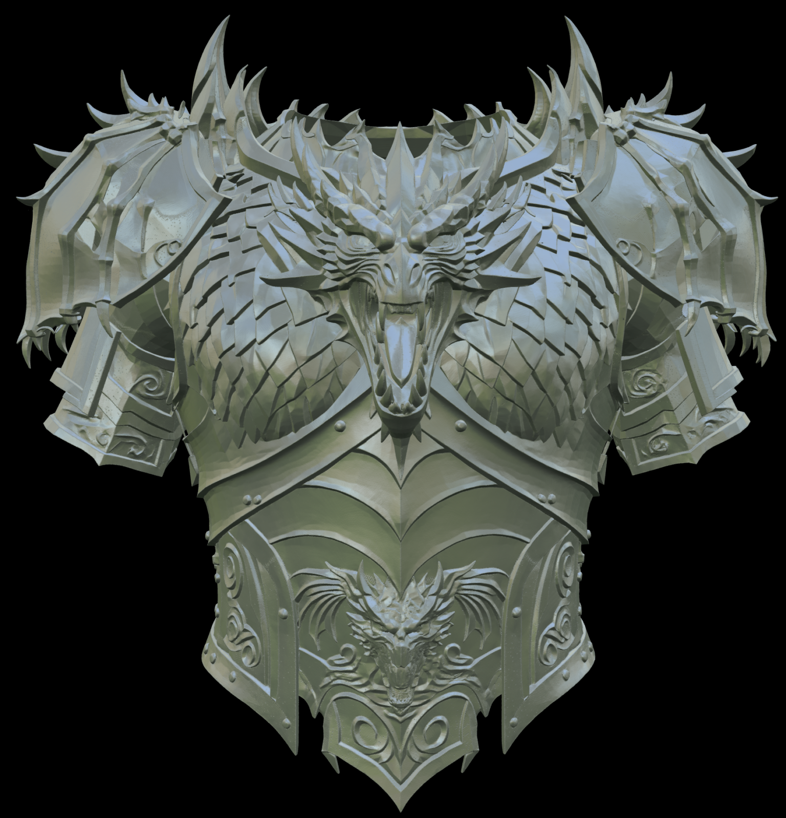
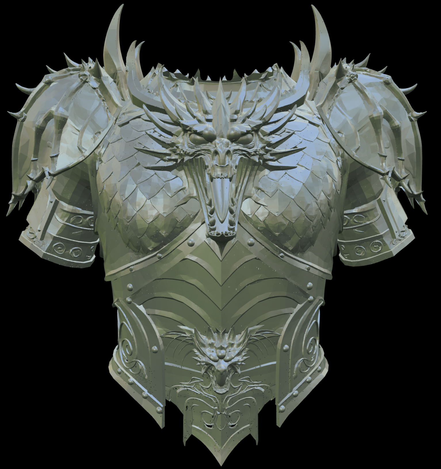
To close, here is a preview of a billion-scale image-to-3D model I am training from scratch, with a release planned for the end of the year. In qualitative comparisons so far, generation has been more consistent than with TRELLIS.2, and the geometry has followed the input image much more closely.