A Deep Dive into 3D Latent Diffusion:
ShapeVAE, Trellis and Hunyuan3D

• Teaser from Trellis, Microsoft's recent state-of-the-art 3D generation model.

Diffusion. From Imagen, DALL·E to Stable Diffusion and Midjourney, Diffusion models have surpassed GANs to become the standard paradigm for modern 2D generative models. In particular, the advent of Latent Diffusion, with its promise of:

"Applying Diffusion in Latent Space → Reduced Computation + High-Resolution Image Generation"

has led to the presentation of 2D generative models that achieve high performance and efficiency, enabling speeds and quality suitable for real-world applications.

The expansion of generative models extends beyond 2D to the realms of video and 3D. In 2024, video generation models such as Sora, DreamMachine (Ray), and Veo have demonstrated the potential for modality expansion.

In recent days, beyond video, latent diffusion-based models are also proving their capabilities in the 3D domain.

This article delves into the concept of 3D Latent Diffusion and analyzes its core component, ShapeVAE, examining how it overcomes the limitations of traditional Score Distillation Sampling (SDS) and NeRF-based Large Reconstruction Models (LRMs). Furthermore, we will compare and contrast the state-of-the-art 3D generation models, Trellis and Hunyuan3D, providing an in-depth exploration of their design differences, strengths, and weaknesses.

Preliminary: What is Latent?

RBF Network	Gaussian Mixture Model	3D Gaussian Splatting

Consider classical machine learning concepts like Radial Basis Function (RBF) networks and Gaussian Mixture Models (GMMs). The core idea of both is to approximate a data distribution (or function) by combining:

• Several basis functions, and
• The weight of each basis function.

$$ f(x) \approx \sum_{i=1}^{N} w_i \phi(||x - c_i||) $$

Equation: Radial Basis Function (RBF)

From a similar perspective, 3D Gaussian Splatting can also be interpreted as approximating data (multi-view observations of a 3D scene) through a combination of:

• Multiple basis functions (3D Gaussian primitives), and
• The weight of each basis function (the opacity of each Gaussian).

$$ \text{Scene}(x) \approx \sum_{i=1}^{N} \alpha_i G_i(x; \mu_i, \Sigma_i) $$

Equation: 3D Gaussian Splatting

Here, the RBF and Gaussian primitives each have learnable parameters (e.g., mean, variance) that are optimized during the learning process.

Shifting our perspective slightly, these basis functions (primitives) can be considered a type of 'latent vector' that compresses the meaning of the data distribution. The entire collection can be viewed as a 'latent vector set'.

RBF networks, 3D Gaussian Splatting, etc., define their basis representations in a human-crafted manner. However, if we learn the basis functions in a learnable way for a given data distribution, this becomes Representation Learning in the context of Deep Learning.

1. ShapeVAE: Representation Learning for 3D Shape

Goal: Representation Learning for 3D Shape

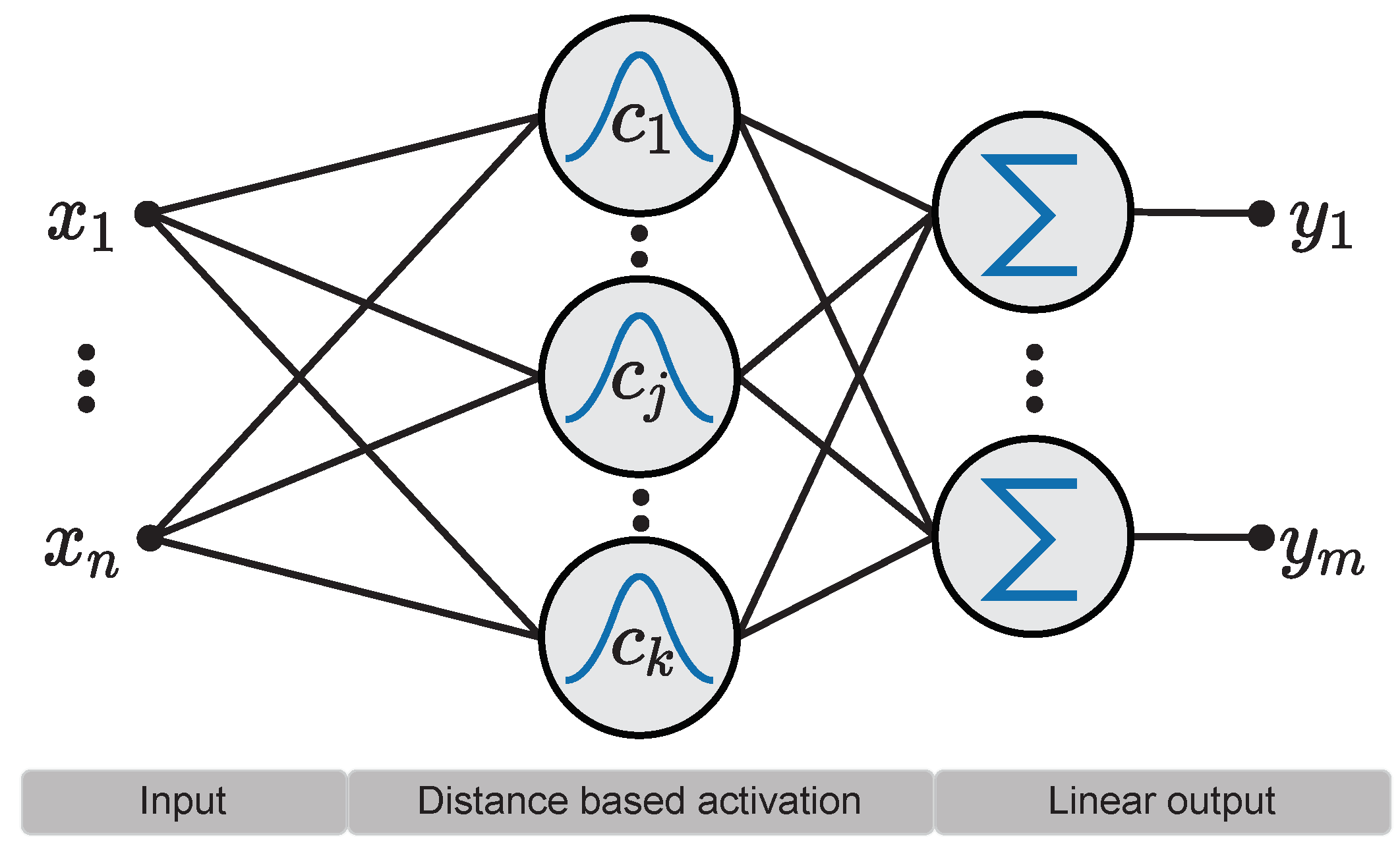
ShapeVAE is an AutoEncoder (specifically, a Variational AutoEncoder or VAE) defined for 3D shapes. Like AutoEncoders (VAEs) in other domains used in Latent Diffusion Models (LDMs), the purpose of all ShapeVAEs is the same:

"To obtain a semantically meaningful, learnable representation of the input data."

Prominent examples include:

• Shape2vecset
• Michelangelo (Neural Carver)
• Craftsman

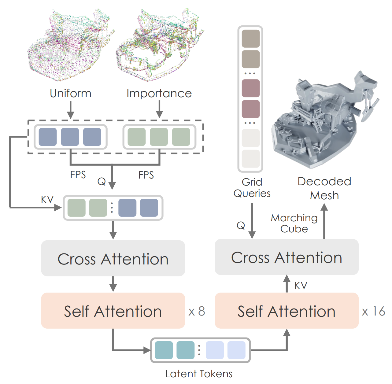
All of these share a similar pipeline design. In essence, it's a standard AutoEncoder structure with the following characteristics:

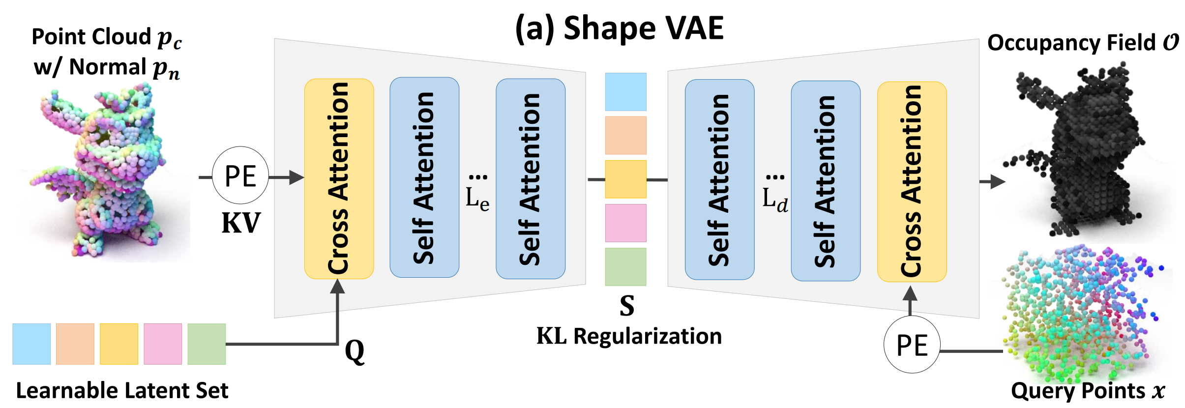
1. Input: Point clouds (usually sampled from the ground truth mesh of the training set).
2. What to Learn? a. Learnable query (latent vector set). b. AutoEncoder (weights of the linear projection layers in each self/cross-attention block).
3. Output: 3D shape, typically represented as occupancy fields (a binary voxel grid).

Here, the learnable query acts as a kind of basis in a compressed, semantically meaningful space (the latent space) representing the data distribution (3D shapes).

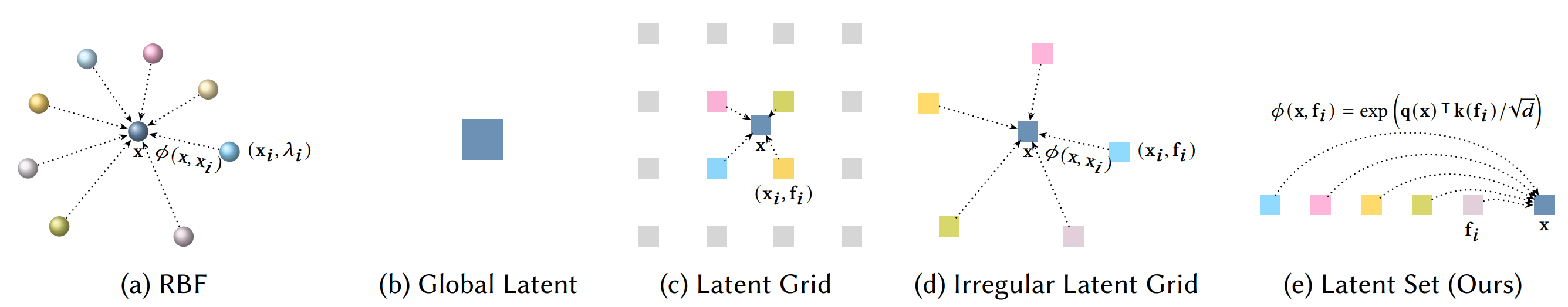
This functions similarly to the kernel basis discussed in the preliminaries.

In ShapeVAE, using the VAE and learnable queries, the similarity of the learnable query (the basis in the latent space) is reflected for a query point $(x)$:

$$ \sum_{i=1}^{M} \mathbf{v}(\mathbf{f}_i) \cdot \frac{1}{Z(\mathbf{x}, \{\mathbf{f}_i\}_{i=1}^{M})} e^{\mathbf{q}(\mathbf{x})^{\mathsf{T}} \mathbf{k}(\mathbf{f}_i) / \sqrt{d}} $$

where Z is a normalizing factor (so, excluding v, it's effectively a softmax). This embedding is then decoded to reconstruct the ground truth shape, thereby learning the latent space.

The authors of Shape2vecset, who first introduced ShapeVAE, state that they drew inspiration from RBFs for this design. Since $q(x)$ is the input embedding, the learnable parameters here are the latent vectors $(f_i)$ and their corresponding weights $(\mathbf{v}(f_i))$. This is analogous to approximating the RBF value using the weighted similarity between the query point and the kernel basis, and then optimizing the basis function using this approximation.

This equation can also be interpreted as a form of QKV cross-attention in a Transformer. The authors define the learnable latent, drawing inspiration from DETR and Perceiver, as follows:

$$ \text{Enc}_{\text{learnable}}(\mathbf{X}) = \text{CrossAttn}(\mathbf{L}, \text{PosEmb}(\mathbf{X})) \in \mathbb{R}^{C \times M} $$

In other words, the ShapeVAE AutoEncoder uses a basis (the latent query, L) to encode and decode the relationship between the basis and each data instance (X).

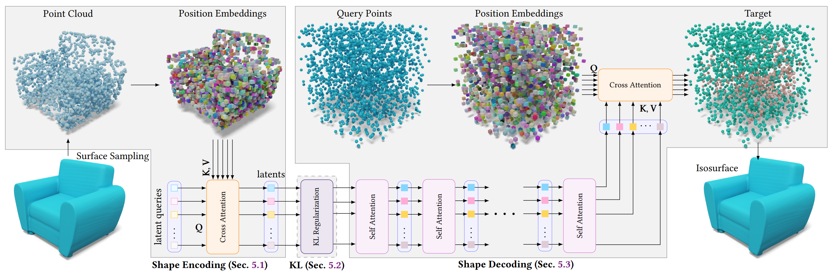
It learns the latent space that best represents the shape, and the basis (learnable query) that best captures the information about that latent space.

The components of the pipeline have the following details:

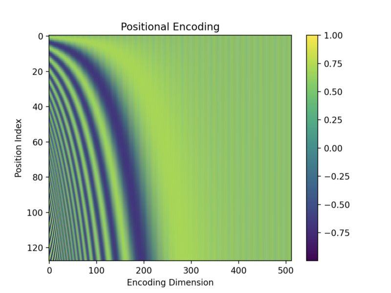
• Positional Encoding: Fourier features, similar to the sinusoidal encoding used in NeRF and Transformers. PE not only maps Cartesian coordinates to a high-dimensional, frequency domain, but also adds stationarity between coordinates when learning kernel regression.
• KL regularization term: Encourages the latent distribution generated by the encoder to be close to the prior distribution (typically a standard Gaussian distribution, $N(0, 1)$). This provides several advantages:
  • Continuous latent space: A latent space following a normal distribution is continuous and smooth, making interpolation and sampling in the latent space easier.
    • Shape variations can be naturally controlled through vector operations (interpolation, extrapolation, etc.) in the latent space.
  • Prevent Overfitting: By constraining the latent space to be close to the prior distribution, the encoder is encouraged to learn the distribution of the training data in a more general form.
  • Sampling Ease: New data can be generated by simply sampling randomly from the standard Gaussian distribution and inputting it to the decoder.

Q. Why learnable query? DETR and Perceiver are fundamentally designed for tasks like detection and classification, not generation. While learnable queries are sometimes used, they are not common in 2D LDMs. However, the reasons for introducing latent queries in ShapeVAE can be inferred as follows:

• Hierarchy: Clear Part-based Structure: 3D shapes often consist of meaningful parts. These parts have spatial relationships and constitute the overall shape.
• Sparsity & Geometry: 3D shapes have sparse characteristics, and the geometry itself is the core information, much sparser than the texture, style, and background of a '2D image'. Therefore, they are well-suited for compression using a latent query approach.

While there are differences in the structure used for the encoder/decoder (Perceiver ↔︎ Diffusion Transformer) and whether additional losses are added for multi-modal alignment in the latent space (CraftsMan), the fundamental role of ShapeVAE remains consistent.

With a well-trained latent space derived from rich data, we can expect that, leveraging the power of Latent Diffusion Models, a generative model for 3D shapes (a 3D Latent Diffusion Model) can be trained.

Challenges for ShapeVAE

However, until recently, 3D generation has not shown the same remarkable results as 2D and video generation. The reasons for this slower progress include:

• Versatility & Diversity of Data: The amount of data is extremely limited compared to 2D. Objaverse, one of the larger datasets, contains around 8 million assets, and even its expanded XL version only has around 100 million, significantly less than 2D datasets (LAION-5B has 5 billion...). High-quality datasets are even more scarce.
• Curse of Dimensionality: Being three-dimensional, generating high-resolution outputs is more computationally expensive than in 2D.
• What is the ‘BEST’ representation? The question of the appropriate representation for '3D' is an open problem without a definitive answer. Besides neural fields, there are numerous representations like voxels, occupancy grids, and SDFs, each with its advantages and disadvantages, making it difficult to choose one.

Furthermore, the popularity of NeRF led to SDS, a combination of 2D Diffusion and NeRF, becoming mainstream in 3D generation. However, it has been extremely difficult to overcome its inherent limitations (extremely slow generation time and the Janus problem). cf: Are NeRF and SDS Destined to be Obsolete in 3D Generation?

The performance of ShapeVAE is directly related to 1) the quantity and diversity of data. Early ShapeVAEs focused more on generative approaches to surface reconstruction than 3D generation, and were therefore trained on limited datasets like ShapeNet. Even when trained on larger datasets, they struggled to faithfully reproduce input images or text.

Another problem with ShapeVAE is that feature aggregation is 'dependent only on spatial location'. Basically, point features in ShapeVAE are input as 'Positional Encoding'. However, Positional Encoding alone is insufficient to capture important 3D information such as local structure (curvature, surface normal) and global shape context (connection relationships between vertices and faces).

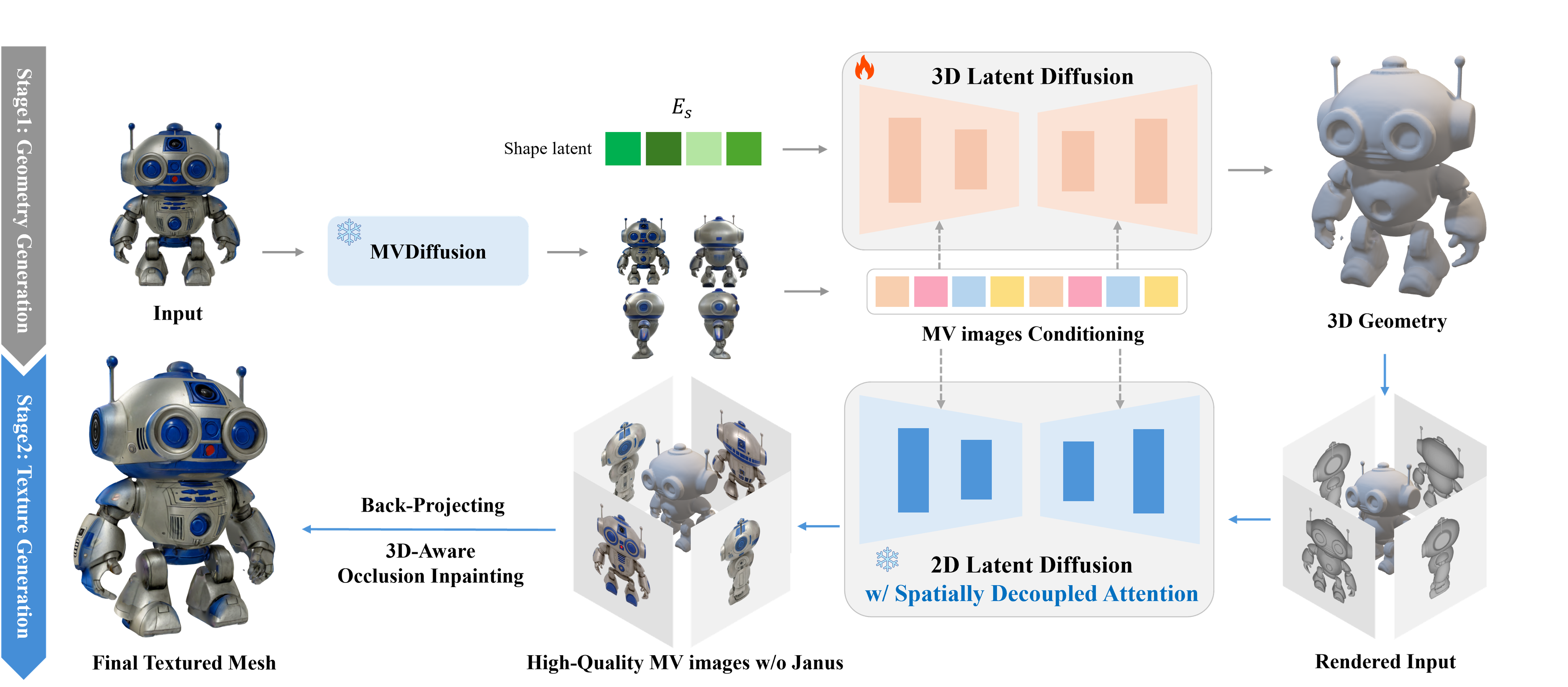
CLAY-Rodin actively utilizes ShapeVAE in the geometry generation stage, greatly increasing model and data capacity, and uses a texture synthesis approach for texture generation.

Rodin significantly improves the performance of ShapeVAE and shape generation in its latent space using a large DiT model (1.5B), and achieves results that surpass previous 3D generation quality by using a two-stage approach of generating a shape (mesh) and then generating texture on it using geometry-guided multi-view generation.

• CaPa, with a similar pipeline to Clay. It generates a mesh with a 3D LDM and then backprojects high-quality texture.

Following this research, the number of studies presenting 3D Latent Diffusion itself gradually increased in 2024. However, the aforementioned problems:

1. Low Quality
2. Not faithfully following the guidance (input image or text)

remained difficult to solve...

2. Trellis

Paper: Trellis: Structured 3D Latents for Scalable and Versatile 3D Generation

Trellis is a state-of-the-art 3D Latent Diffusion model announced by Microsoft in late 2024. It significantly outperforms previous ShapeVAE-based approaches in terms of instruction following and stability, and has the advantage of generating both shape and texture end-to-end. Let's analyze the design that enabled it to achieve state-of-the-art quality.

2.1. Structured Latent Representation

The authors propose a representation called SLAT (Structured Latent Representation):

$$ \mathbf{z} = \{(\mathbf{z}_i, \mathbf{p}_i)\}_{i=1}^{L}, \quad \mathbf{z}_i \in \mathbb{R}^{C}, \quad \mathbf{p}_i \in \{0, 1, \dots, N-1\}^3, $$

where $p_i$ is the voxel index and $(z_i)$ is the latent vector. That is, each voxel grid has a latent vector assigned to it, and the latent vector set itself is structured (voxelized), hence the name SLAT.

Due to the sparsity of 3D data, the number of activated grids is much smaller than the total size of the 3D grid $(L << N^3)$, which means that relatively high-resolution outputs can be generated. This approach is similar to voxel-grid NeRFs like Instant-NGP, but uses ShapeVAE to predict the featured voxel-grid.

While the definition itself might seem like simply mapping the learnable query used in ShapeVAE to a voxel grid, the core of SLAT is that it actively utilizes the DINOv2 feature extractor during the learning process of this SLAT encoding.

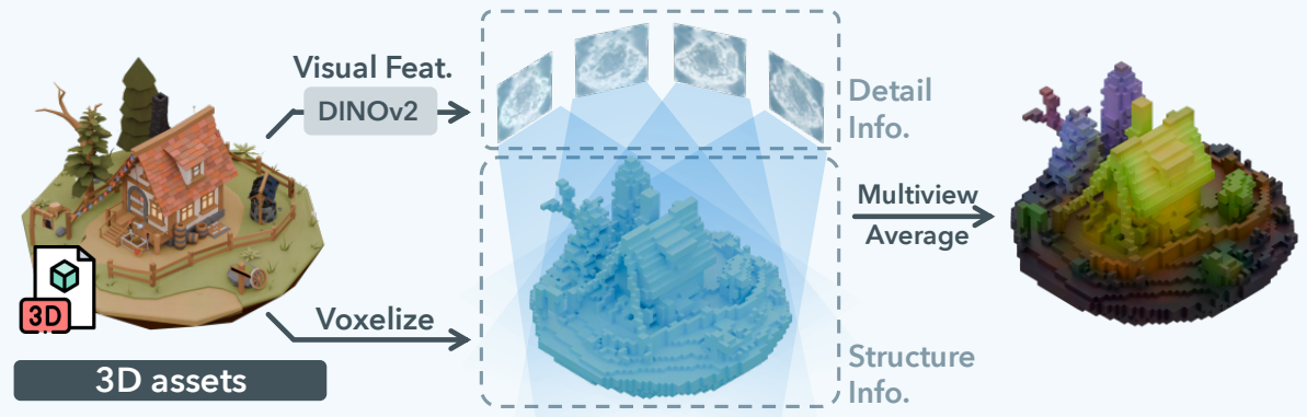
As shown in the figure above, SLAT calculates the encoding for 3D assets during the VAE training process by:

1. Multi-View Rendering.
2. Featurizing: Extracting features for each view rendering using DINOv2.
3. Averaging.

In other words, Trellis overcomes the limitations of ShapeVAE stemming from the 'PE-only input feature encoding' by utilizing a well-trained 2D feature extractor (DINOv2).

This approach seems to be adopted because Trellis aims for end-to-end 3D generation. It obtains versatile features using pre-trained DINOv2 to capture information about 3D assets, such as color and texture, which are difficult to represent with PE alone.

The VAE structure itself is the same as the original ShapeVAE. Since the latent space is well-defined, the decoder can be changed to fine-tune the output to generate 3D Gaussian Splattings (GSs), Radiance Fields (NeRFs), or Meshes. Therefore, Trellis can predict outputs in a format-agnostic manner, including GSs, NeRFs, and Meshes. (The actual inference branch uses both GS and Mesh branches).

2.2. SLAT Generation

Q. So, can new assets be generated by simply inputting a random sample from a Standard Gaussian Distribution in the latent space, as in ShapeVAE?

Unfortunately, this is not the case. First, since SLAT's 'structure' (position index) itself is meaningful, it is necessary to generate the structure, i.e., which voxels are empty and which are not.

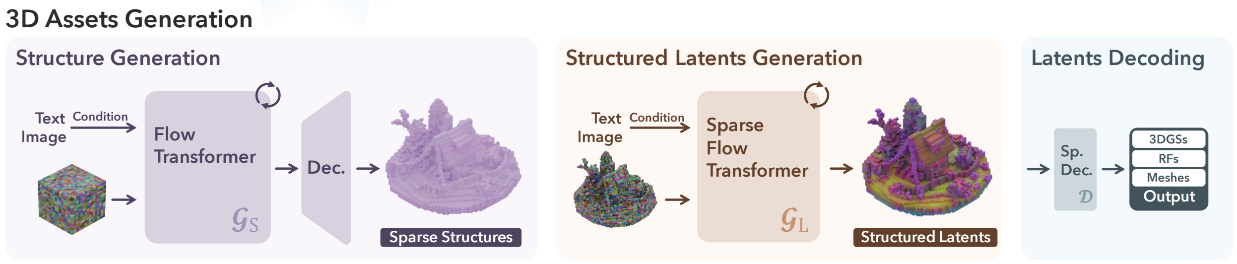
To achieve this, Trellis uses a two-stage approach in 3D generation.

1. Generate Sparse Structure via Conditional Flow Matching: Uses a rectified flow model. (model 1) $$ \mathcal{L}_\text{CFM}(\theta) = \mathbb{E}_{t, \mathbf{x}_0, \epsilon} || \mathbf{v}_\theta(\mathbf{x}, t) - (\epsilon - \mathbf{x}_0) ||_2^2. $$
2. Generate the final SLAT using a Transformer similar in structure to DiT, with the generated Sparse Structure as input. (model 2)

Directly generating the structure as a dense grid in the first stage is computationally expensive. Therefore, Trellis also adopts a Decoder in the Structure Generation Stage, generating a low-resolution feature grid and then scaling it up with the Decoder.

The ground truth dense binary grid $\mathbf{O} \in \{0, 1\}^{N \times N \times N}$ is compressed into a low-resolution feature grid $\mathbf{S} \in \mathbb{R}^{D \times D \times D \times C_s}$ using 3D convolution. A Flow Transformer is then trained to predict this compressed representation.

Because $\mathbf{O}$ is a coarse shape, there is almost no loss during the compression process using 3D convolution, which also improves the efficiency of neural network training. Furthermore, the binary grid of $\mathbf{O}$ is converted to continuous values, making it suitable for Rectified Flow training.

The Rectified flow model employs linear interpolation (input → output) of the straight-line path from data → noise as the forward process in the diffusion process. Compared to inefficient steps in typical Neural ODE solvers, Rectified Flow can model the linear vector field from data → noise, enabling much faster and more accurate generation.

In this process, condition modeling is performed similarly to other Diffusion models, injecting into the KV of cross-attention. In other words, Sparse Structure Generation acts as a kind of Image/Text-to-3D Coarse Shape Generation.

Subsequently, model 2, which generates SLAT using the generated Sparse Structure, is also trained using Rectified Flow. The decoder of ShapeVAE is then used on the finally generated SLAT to produce GSs / Mesh outputs.

The final 3D asset output uses RGB representation for GS generation results and geometry for Mesh generation results, fitting the mesh texture to the GS rendering. This is likely a strategy employed because it is difficult to convert 3D GS into a clean mesh.

Specifically, the steps are:

1. Multi-view Rendering: Rendering the GSs generation results for a predetermined number of views.
2. Post-processing: Post-processing the Mesh generation results using the mincut algorithm for retopology, hole filling, etc.
3. Texture Baking: Learning the texture by minimizing the Total-Variation Loss (L1) between the mesh texture and the multi-view GS renderings from step 1) (using them as ground truth textures), and finally baking the texture onto the Mesh.

The glb outputs available for download on the demo page are all the results of this pipeline.

• cf: to_glb, fill_holes

It demonstrates outputs of impressive quality. On the project page and Demo, you can see results that are even better than the paper captures.

A drawback is that it doesn't yet completely follow instructions (input guidance) perfectly, and perhaps because the default branch of the decoder is GSs, the quality of the generated mesh isn't always excellent.

3. Hunyuan3D-v2

Paper: Hunyuan3D 2.0: Scaling Diffusion Models for High Resolution Textured 3D Assets Generation

After the emergence of Trellis, it seemed that Trellis would firmly hold the throne of SOTA 3D Generation for some time. However, Hunyuan3D-v2 from China has appeared, surpassing Trellis in terms of Mesh Quality and Instruction Following.

Unlike Trellis, Hunyuan3Dv2 is not end-to-end but follows a two-stage approach like Rodin or CaPa: 1) Mesh Generation 2) Texture Generation. The Mesh Generation quality is truly SUPERIOR. Let's analyze it in detail.

3.1. Hunyuan-ShapeVAE

The design of Hunyuan's ShapeVAE is not very different from vanilla ShapeVAE, but there are some significant differences:

1. Point Sampling: When training ShapeVAE, point clouds are usually obtained from the ground truth mesh through uniform sampling. However, this often leads to the loss of fine details. Therefore, Hunyuan uses a point sampling strategy that focuses more on edges and corners, in addition to uniform sampling. This approach is similar to that of the recently proposed Dora.

   

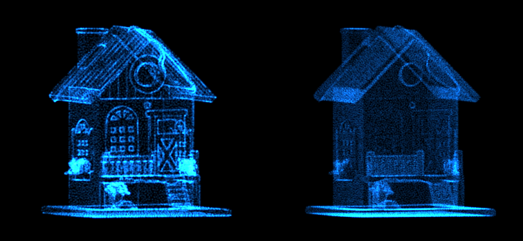
   Figure from Dora. Left: salient points ↔︎ Right: uniform

2. SDF estimation: The VAE output is not a binary voxel grid but SDF values. Unlike the existing occupancy method, which requires predicting a binary grid, this allows the deep learning model to estimate continuous real SDF values, resulting in more stable outputs.

3. Point Query: It does not use the strategy of learnably learning the basis of the latent space as a latent vector set. Instead, it uses salient/uniform sampled points, subsampled, as queries.

   

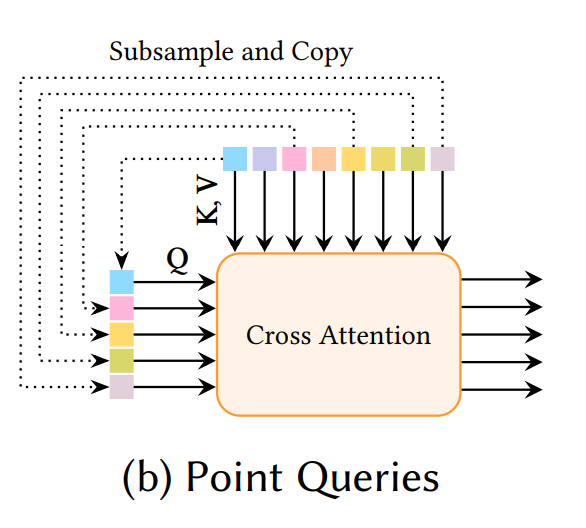
It seems they have adopted a strategy of learning the latent space itself more precisely, rather than learning the basis of the latent space. This approach is likely possible because salient sampling sufficiently reflects the fine details of each 3D shape.

• Figure: Hunyuan-ShapeVAE

3.2. Hunyuan3D-DiT

The core of Hunyuan3D-DiT is the novel architecture design of the 3D generation stage.

Previous studies, including Trellis, used Transformers not significantly different from the general DiT structure. However, Hunyuan uses a 'double- and single-stream' design like Flux.

Although there is no official technical report for Flux, according to the released development version code, it processes information from the text ↔︎ image modalities in a double-stream manner. This is considered the main reason why Flux achieves better instruction-following performance compared to SDXL.

SDXL	Flux

• cf. unofficial diagram of Flux Pipeline
• My opinion) The structure of the double stream is similar to the reference net method of ControlNet. I suspect it was inspired by the way ControlNet effectively reflects conditions without compromising the generation capability of the original modal.

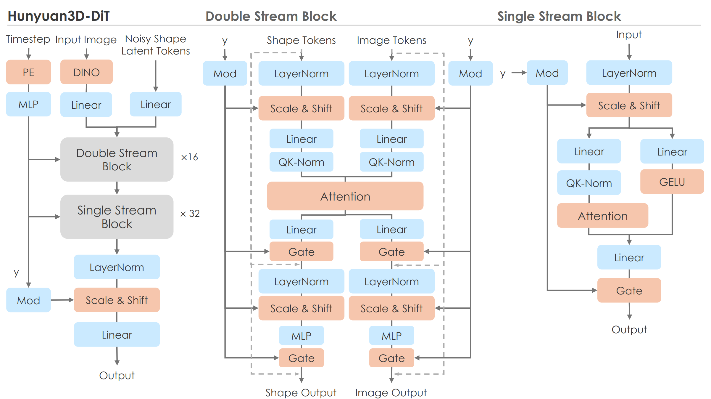
Hunyuan also adopts this 'double-single' structure to generate high-quality 3D shapes while preserving as much information as possible from the condition (image, text) instructions.

The core of the pipeline is as follows:

• Double Stream:
  • Shape Tokens: Latent representation tokens (noisy) of the 3D shape to be generated are refined through the diffusion reverse process of DiT.
  • Image Tokens: 2D image features extracted from the input image (image prompt) using pre-trained DINOv2.
  • Shared Interaction: Shape and Image Tokens are processed through separate paths, but interactions between the two tokens are reflected within the Attention operation. This effectively incorporates information from the image prompt into the 3D shape generation process.
• Single Stream:
  • Input: Shape Tokens that have incorporated image information through the double-stream.
  • Output: The tokens are processed independently to further refine the 3D shape latent representation and generate the final 3D shape (latent).

Training, like Trellis, reportedly uses Rectified Flow Matching.

$$ \mathcal{L} = \mathbb{E}_{t, x_0, x_1} \left[ || u_\theta(x_t, c, t) - u_t ||_2^2 \right] $$

Among the mentioned training details, it is noteworthy that unlike ViT-based approaches that typically add positional embedding (PE) to each patch, Hunyuan removed PE. This is to prevent specific latents from being assigned to 'fixed locations' during shape generation.

3.3. Hunyuan3D-paint

Since Hunyuan uses a 2-stage approach like CLAY/CaPa, it uses Geometry-guided Multi-View Generation for texture synthesis. However, it is not simply a combination of MVDream/ImageDream series models + MV-Depth/Normal ControlNet. Instead, it incorporates several novel strategies to improve quality.

First, Hunyuan starts by pointing out the problems with existing methods. MVDream and ImageDream try to achieve Multi-View Synchronization in the generation branch using 'noisy features' while tuning the Stable Diffusion model for Multi-View. This can lead to the loss of original details in the reference image. Indeed, looking at the MV output of ImageDream or Unique3D, even the front view often shows degraded quality compared to the input image.

input	generated front view (MVDiffusion)

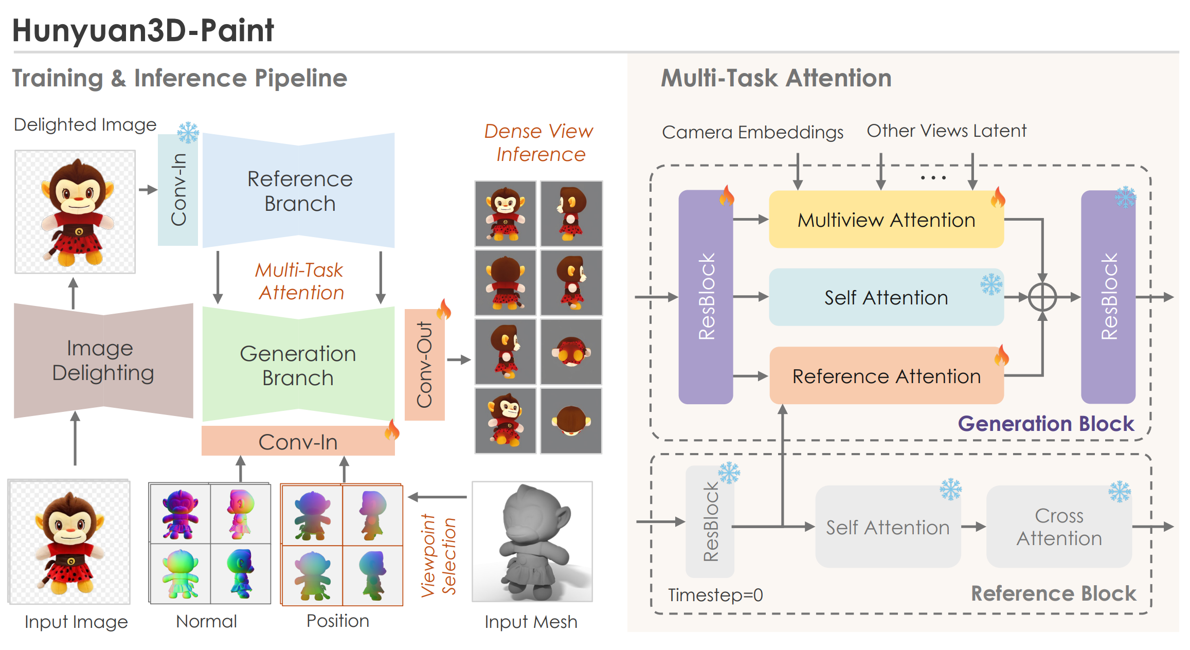
To address the shortcomings of existing MVDiffusion, Hunyuan uses the following approaches:

• Clean Input Noise

  • The "original VAE feature" (clean VAE feature without noise) of the reference image is directly injected into the reference branch to preserve the details of the reference image as much as possible.
  • Since the feature input to the reference branch is noiseless (clean, input of the forward process), the timestep of the reference branch is set to 0.

• Regularization & Weight Freeze Approach

  • Style Bias Regularization: To prevent style bias that may occur in datasets rendered from 3D assets, they reportedly abandoned the shared-weighted reference-net structure.
  • Weight Freeze: Instead, the weights of the original SD2.1 model are frozen and used as a reference-net. The SD2.1 model serves as the base model for multi-view generation, and the 'frozen weights act as a regularization'. This is a similar strategy to MVDream, where about 30% of the generation results were trained with a simple text-to-image (not MV) loss (from the LAION dataset) to preserve the fidelity of the MVDiffusion model.

  This might be a bit confusing, but think of it as using the opposite approach of typical ControlNet. The reference branch, which plays the control role, is not trained, and the generation branch (MV-Diffusion model) is trained. The 'guide' is handled by the original SD model, and 'gen' is handled by the MV-Diffusion model.

• For Geometry Conditioning, both of the following are used:

  • CNM (Canonical Normal Maps): An image of the 3D model surface normal vectors projected onto a canonical coordinate system.
  • CCM (Canonical Coordinate Maps): An image mapping the 3D model surface coordinate vectors to a canonical coordinate system.

  Both project onto a canonical system to provide geometry-invariant information. Using both coordinate and normal information maps both the spatial position and the relationships between positions. MetaTextureGen also uses the same guidance, reporting that the combination of point and normal is better than depth maps in terms of detail and global context.

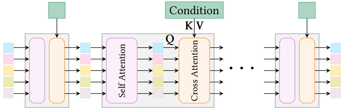
Finally, Multi-Task Attention is proposed to train this structure effectively.

Mathematically, this can be expressed as:

$$Z_{MVA} = Z_{SA} + \lambda_{ref} \cdot \text{Softmax}\left(\frac{Q_{ref} K_{ref}^T}{\sqrt{d}}\right) V_{ref} + \lambda_{mv} \cdot \text{Softmax}\left(\frac{Q_{mv} K_{mv}^T}{\sqrt{d}}\right) V_{mv} $$

As the equation indicates, this is a parallel attention mechanism designed for a form of "multi-task learning," where the reference (Ref) module and the multi-view (mv) module operate independently.

This design is motivated by the distinct roles of the reference branch (ControlNet) and the generation branch (MV generation) in the current architecture:

• Reference branch: Aims to adhere to the original image.
• Generation branch: Aims to maintain consistency between generated views.

The Multi-Task Attention mechanism is intended to mitigate the conflicts and resulting performance degradation that can arise from this multi-functionality.

A similar structural design has been demonstrated in MV-Adapter. Both cases employ this design to achieve multi-view generation capabilities without sacrificing the performance of the original branch. In a sense, this approach is analogous to the double-stream architecture of the ShapeGen stage.

This architecture enables a diffusion model design that leverages the reference image as guidance while simultaneously ensuring multi-view consistency. In other words, it allows for the generation of natural images from various viewpoints while maintaining consistency with the reference image.

Tests have shown that this approach produces MVDiffusion outputs with quality significantly surpassing the fidelity of existing MVDiffusion methods. Furthermore, it exhibits higher multi-view consistency and fewer seams and artifacts compared to competitors that rely solely on normal or depth maps for guidance.

• Figure from MV-Adapter. An ablation study demonstrating the effectiveness of the parallel structure.

In my own testing, truly superior-quality meshes were generated, and the geometry-guided MV Diffusion results also exhibited higher fidelity and consistency than any previous model I've encountered.

Test results showed MVDiffusion output quality that overwhelmingly surpasses the fidelity of existing MVDiffusion, and it exhibited higher multi-view consistency and fewer seams and artifacts than competitors that simply use normal/depth maps as guides.

Hunyuan	ImageDream

4. Trellis vs Hunyuan?

Trellis	Hunyuan

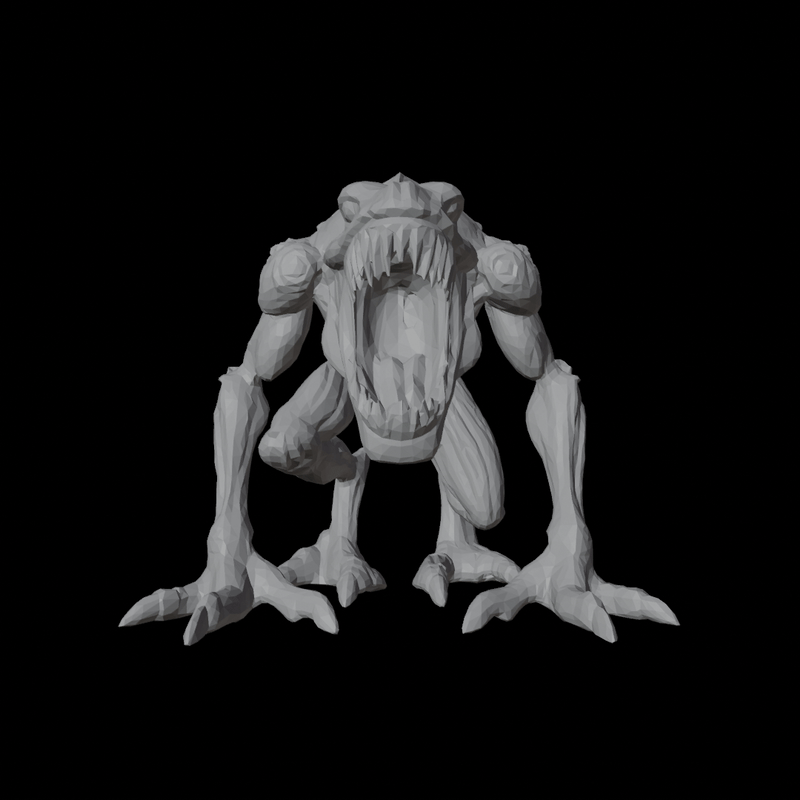
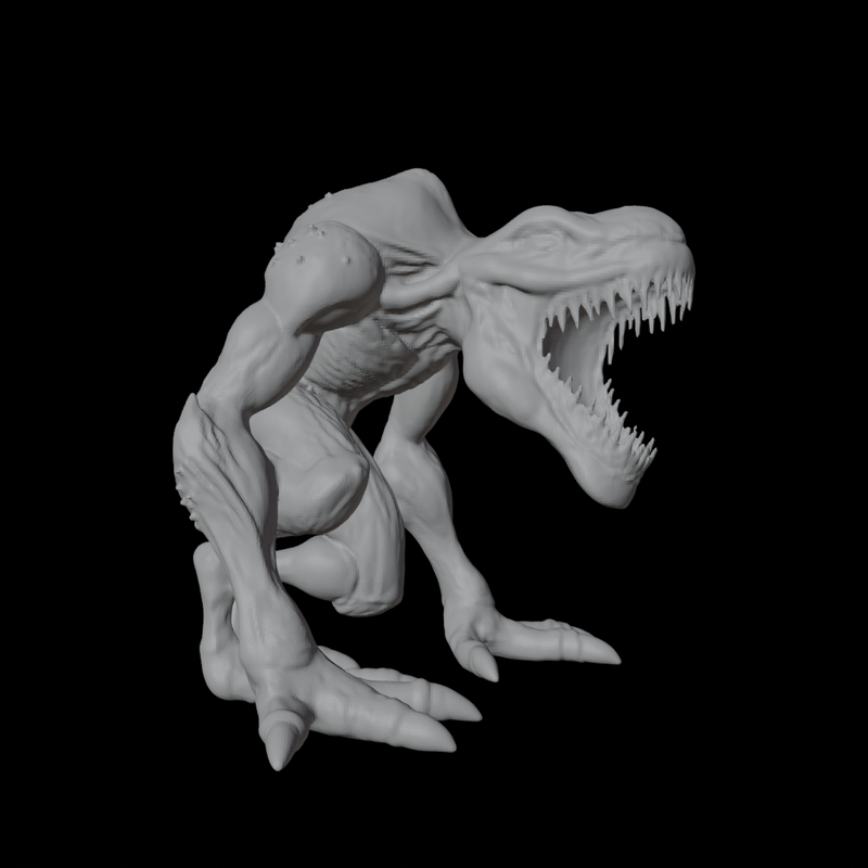
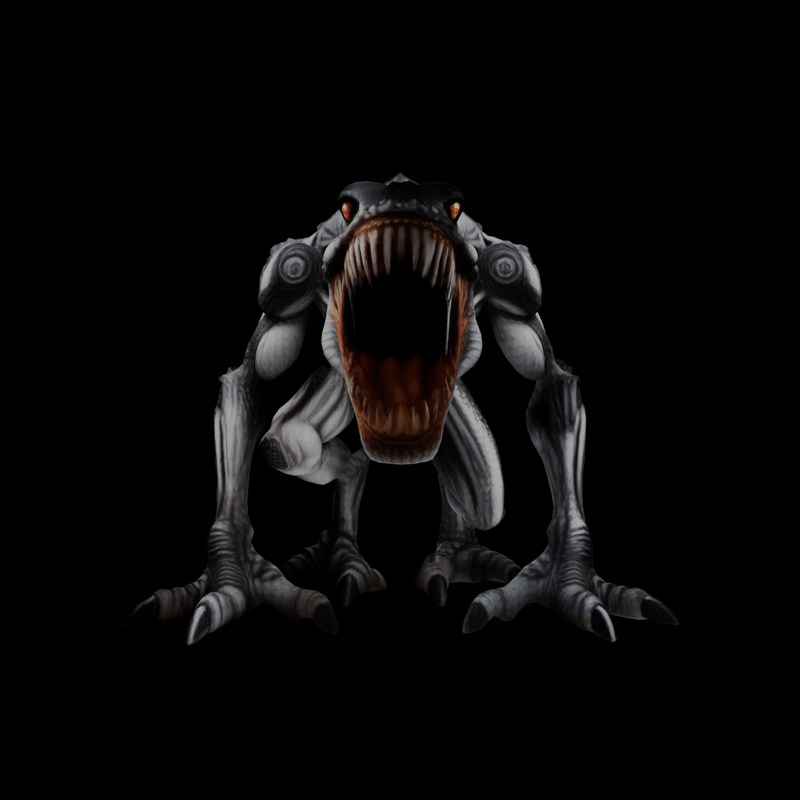
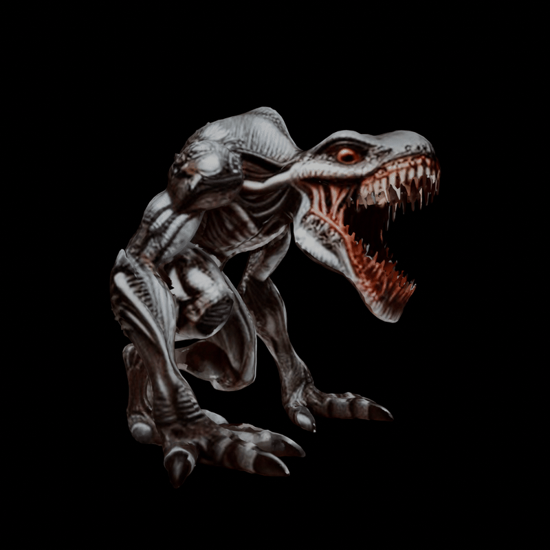
During my own tests, in terms of Mesh Quality, Hunyuan3D's topology is significantly better than Trellis. Furthermore, although not included in the blog post, Trellis sometimes predicts results that differ from the input image guidance, while Hunyuan consistently demonstrates faithful instruction following.

On the other hand, Texture Quality is not yet very high for either model. Hunyuan generates textures by generating 6 view Multi Views geometry-guided and backprojecting them, which tends to result in some occlusion. Trellis exhibits less occlusion than Hunyuan, but its fidelity is comparatively worse. Additionally, in the case of Hunyuan, it does not perfectly align with the geometry guide, sometimes making seams or artifacts more noticeable than in Trellis.

The clear advantages and disadvantages seem to arise from their respective end-to-end vs. 2-stage pipelines. It is anticipated that subsequent research in 3D Latent Diffusion will emerge, enhancing quality in each of these aspects.

Finally, I show CaPa's Result :)

Closing

Thus far, I have provided a detailed analysis tracing the evolution of state-of-the-art 3D Latent Diffusion, from the fundamental concepts of ShapeVAE to Trellis and Hunyuan3D.

While the open-source community did not achieve remarkable progress in the 3D field for some time after the emergence of CLAY, recent studies have showcased innovative designs and reached state-of-the-art quality, further fueling anticipation for generative models in the 3D domain.

Personally, Hunyuan's application of proven designs from Flux, MV-Adapter, and other works to the 3D generation scheme is particularly impressive. It reinforces the notion that to conduct impactful research, one must remain attentive to research trends in other fields.

Finally, recent research, led by MeshAnything, is attracting attention by focusing on the auto-regressive generation of mesh faces to create what are termed "Artistic-Created Meshes" (these studies also utilize the ShapeVAE latent space). However, due to its auto-regressive nature, this approach is time-consuming, and the quality is not yet satisfactory; therefore, it seems prudent to observe its development for the time being.