Introduction
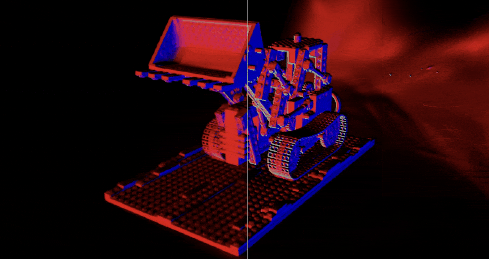
This article provides an in-depth review of the paper "2D Gaussian Splatting for Geometrically Accurate Radiance Fields," which introduces a novel approach to generating real-world quality meshes. Before diving into the review, I present an impressive result from the Lego scene in the NeRFBlender dataset, created using 2D Gaussian Splatting (2D GS). It's quite something!

Challenges in Mesh Reconstruction for Radiance Fields
In a previous discussion (Can NeRF be used in game production? (kor)), I highlighted the ongoing challenges in the practical application of Radiance Fields technologies.
Although 3D Gaussian Splatting (3D GS) offers better portability to game and graphics engines compared to NeRF, it still faces significant challenges in mesh reconstruction.
This difficulty arises due to the nature of 3D GS, which resembles a variant of point cloud representation, making it inherently more complex to convert into a mesh than NeRF.
Recently, at SIGGRAPH 2024, "2D Gaussian Splatting for Geometrically Accurate Radiance Fields" stands out as it demonstrates practical usability in mesh generation through a splatting-based approach. Let’s take a look at what 2D GS is!
Recap. Radiance Fields 의 Mesh Recon 의 어려움
1. Background
1.1. 3D Gaussian Splatting

3D Gaussian Splatting is a technique that reconstructs a 3D scene using a set of anistropic & explicit primitive kernel.
3D Gaussians. The original authors of 3D GS defined the covariance matrix of these 3D Gaussians as a density function for a point $p$ in space, using the Gaussian rotation matrix $R$ and scale matrix $S$.
3D GS, by definition, is similar to dense point cloud reconstruction but reconstructs space as explicit radiance fields for novel view synthesis. This explicit representation offers several advantages:
-
Speed
Unlike NeRF, which requires querying a multi-layer perceptron (MLP) to obtain information, 3D GS stores the information of the 3D Gaussians explicitly, enabling real-time scene rendering at over 100 fps without the need to query an MLP. -
Portability
Since 3D GS requires only rasterization, it is much easier to port to game engines and implement in web viewers compared to NeRF. (cf. SuperSplat) -
Editability
3D GS allows for straightforward scene editing, such as selecting, erasing, or merging specific elements within a trained scene, which is more complex with NeRF due to its reliance on MLPs.
1.2. Surface Reconstruction Problem in 3D GS
Despite the advantages, 3D GS presents significant challenges in surface reconstruction. The paper on 2D GS discusses four main reasons why surface reconstruction is difficult in 3D GS:
-
Difficulty in Learning Thin Surfaces
The volumetric radiance representation of 3D GS, which learns the three-dimensional scale, struggles to represent thin surfaces accurately. -
Absence of Surface Normals
Without surface normals, high-quality surface reconstruction is unattainable. While INN addresses this with Signed Distance Functions (SDF), 3D GS lacks this feature. -
Lack of Multi-View Consistency
The rasterization process in 3D GS can lead to artifacts, as different viewpoints result in varying 2D intersection surfaces. i.e., Artifacts!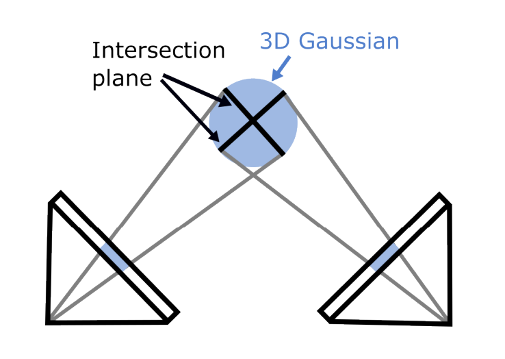
-
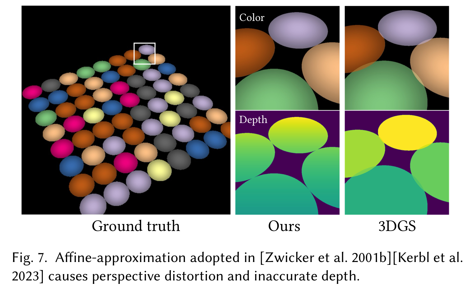
Inaccurate Affine Projection
The affine matrix used to convert 3D GS to radiance fields loses perspective accuracy as it deviates from the Gaussian center, often leading to noisy reconstructions.
Additionally, 3D GS shares NeRF's challenge of generating high-quality meshes through methods like Marching Cubes or Poisson Reconstruction, due to its volumetric opacity accumulation.
1.3. SuGaR: Surface-Aligned Gaussian Splatting
SuGaR (Surface-Aligned Gaussian Splatting) is a previous work that addresses some of the surface reconstruction challenges in 3D GS. SuGaR's core idea is based on the assumption that for well-trained 3D Gaussians, the axis with the shortest scale will align with the surface normal. This approximation is used as a regularization technique to ensure the 3D GS surface is aligned.
However, SuGaR is a two-stage method that first learns the 3D GS and then refines it, leading to a complex learning process. Moreover, it does not fully resolve the projection inaccuracies that contribute to surface reconstruction difficulties, often resulting in meshes with suboptimal geometry in custom scenes.
2. 2D Gaussian Splatting
2.1. 2D Gaussian Modeling (Gaussian Surfels)
The approach of 2D Gaussian Splatting (2D GS) essentially reverses the intuition behind SuGaR: instead of flattening 3D Gaussians to align them with surfaces, learns a scene composed of flat 2D Gaussians, known as surfels.
The Rotation Matrix $R$ and Scale Matrix $S$ for 2D GS can be defined accordingly.
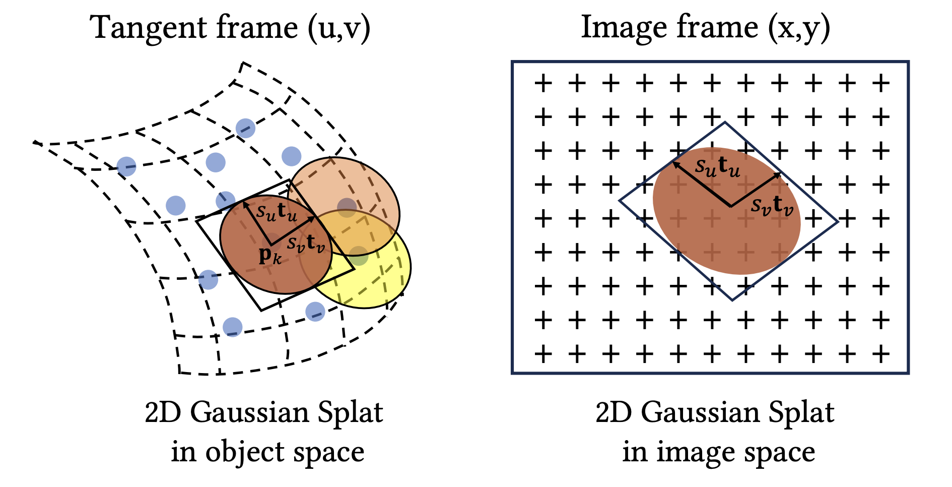
In this context, a 2D Gaussian is defined as a local tangent plane $P$ in the $uv$ coordinate frame which has center point $p_k$, tanget vector $(t_u, t_v)$.
Therefore, the 2D Gaussian is represented by a standard normal function.
The primary parameters to be learned in 2D GS include the rotation axis, scaling, and spherical harmonics coefficients for opacity and non-Lambertian color.
2.2. Splatting
2D-to-2D Projection
In principle, a 2D Gaussian can be used as a 3D GS projection by simply setting the third scale dimension to zero. However, the affine projection method used in 3D GS, based on the first-order Taylor expansion $\Sigma' = JW\Sigma W^{\rm T}J^{\rm T}$, induces approximation errors as the distance from the Gaussian center increases.
related discussion in official repo:

To address these inaccuracies, the authors of 2D GS propose using a conventional 2D-to-2D mapping in homogeneous coordinates.
For a world-to-screen transformation matrix $\mathbf{W} \in \mathbb{R}^{4 \times 4}$, a 2D point $(x,y)$ in screen space can be derived as follows:
This means that the c2w direction ray from a point in camera space intersects the 2D splats at depth $z$, and the Gaussian density of the screen space point can be obtained as
However, the inverse transform can introduce numerical instabilities, leading to optimization challenges.
Ray-Splat Intersection w/ Homography
The authors resolve the ray-splat intersection problem by identifying the intersection of three non-parallel planes.
For a given image coordinate $(x, y)$, a ray is defined as the intersection between two homogeneous planes, $\mathbf{h}_x = (-1, 0, 0, x)$ and $y$-plane $\mathbf{h}_y = (0, -1, 0, y)$. And the intersection is calculated by transforming the homogeneous planes $\mathbf{h}_x$, $\mathbf{h}_y$ to $uv$-space.
By homography, the two planes $\mathbf{h}_u$ and $\mathbf{h}_v$ in $uv$-space are used to find the intersection point with the 2D Gaussian splats.
This closed-form solution provides the projection value from the $uv$-space for the screen pixel, with the depth $z$ obtained from a previously defined equation.
Comparative figures in the supplementary material of the paper demonstrate that the homogeneous projection method in 2D GS is more accurate than the affine projection used in 3D GS.
2.3. Training 2D GS
In addition to the image rendering loss defined through 2D projection and rasterization, the training process for 2D GS incorporates two additional regularization losses: Depth Distortion Loss and Normal Consistency Loss.
Depth Distortion Regularization
Unlike NeRF, where volume rendering accounts for distance differences between intersecting splats, 3D GS does not, leading to challenges in surface reconstruction.
To address this, the authors introduce a depth distortion loss, which concentrates the ray weight distribution near the ray-splat intersection, similar to Mip-NeRF360.
Here, for ray-splat inersection, each variable represents followings:
- $\omega_i = \alpha_i \hat{G}_i(u(x)) \prod_{j=1}^{i-1}(1 - \alpha_j \hat{G}_j(u(x)))$ : blending weight
- $z_i$: depth
The definition of weight shows that it is the same expression as the accumulated transmittance of the NeRF, and by the same logic, when a point is transparent along the current ray direction and the opacity value of the point is high, the weight will be a large value.
In other words, the loss is a regularization that reduces the depth difference between ray-splat intersections with high opacity.
where $A_i = \sum_{j=0}^{i} \omega_j$, $D_i = \sum_{j=0}^{i} \omega_j m_j$, and $D_i^2 = \sum_{j=0}^{i} \omega_j m_j^2$
Also, the implementation of this loss shows that, each of the terms is either an accumulation of opacity or an accumulation of opacity $\times$ depth.
Therefore, this loss can be computed as if it were an image rendering, using the above formula. In the 2D GS implementations, this is handled by the rasterizer.
Normal Consistency Regularization
In addition to distortion loss, 2D GS presents normal consistency loss, which ensures that all 2D splats are aligned with the real surface.
Since Volume Rendering allows for multiple translucent 2D Gaussians (surfels) to exist along a ray, the authors consider the area where the accumulated opacity reaches 0.5 to be the true surface.
They propose a normal consistency loss that aligns the derivative of the surface's normal and depth in this region as follows:
where
- $i$ is the index of the splats intersecting along the ray
- $\omega_i$ is the blending weight of ray-splat intersections
- $\mathbf{n}_i$ is the normal vector of splats
- $\mathbf{N}$ is the normal vector estimated from points in the neighboring depth map.
Specifically, $\mathbf{N}$ is computed using finite difference as follows.
This loss aligns the derivative of the surface's normal and depth in this region, ensuring consistency between the normal vector of splats and the normal vector estimated from the neighboring depth map.
3. Experimens & Custom Viewer
3.1. Qualitative Results
Although the quantitative results on Novel view synthesis may not appear impressive in comparison to previous studies, the true value of 2D GS lies in its qualitative evaluation and practical testing. The performance of 2D GS in surface and mesh reconstruction surpasses that of any previous work.
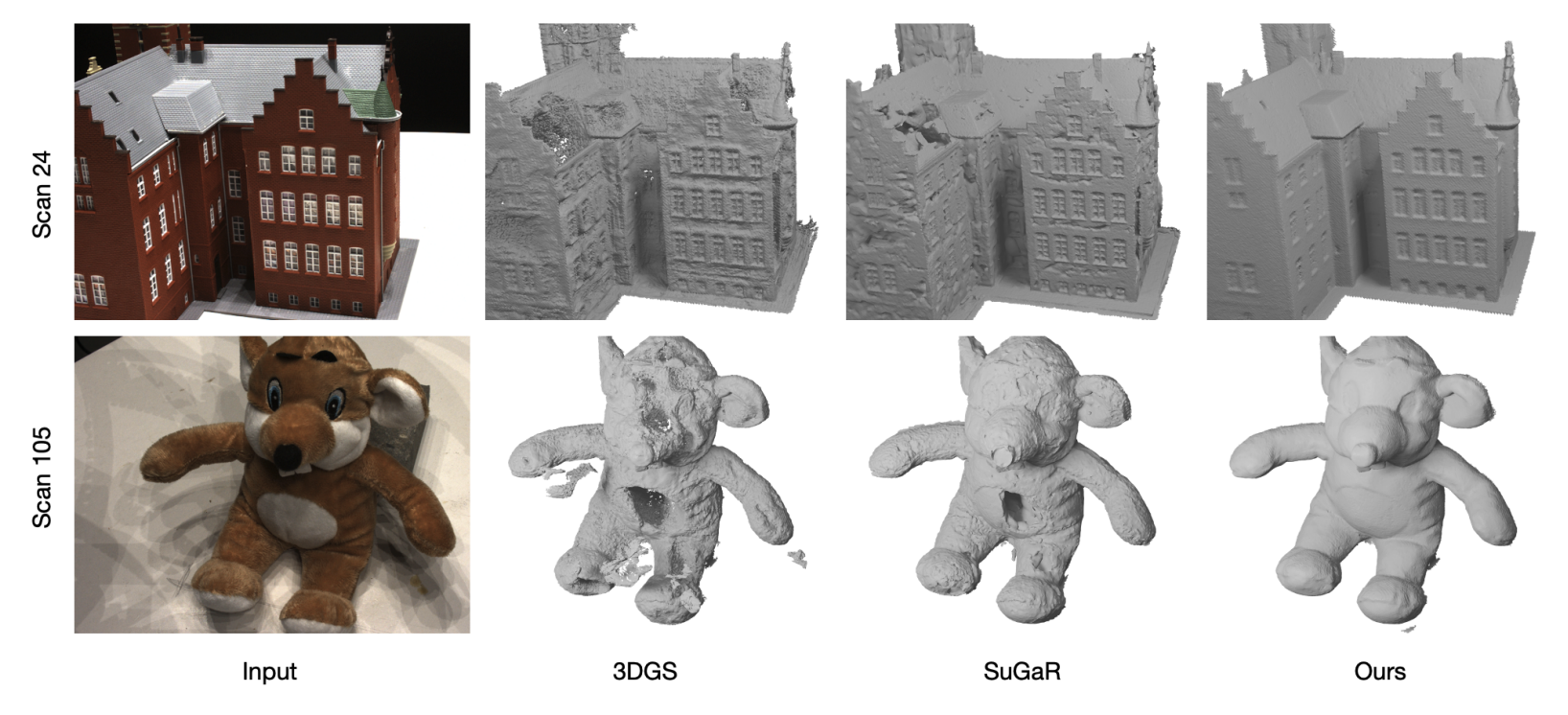
This high performance extends to real-world custom scenes. Experimental results on two custom objects, a guitar, and a penguin.
2D GS: guitar (mesh)
2D GS: penguin (mesh)
It demonstrates that 2D GS can generate meshes of sufficient quality for use in games and modeling, provided that issues related to light condition disentanglement are addressed.
Moreover, 2D GS's ability to accurately extract depth values enables quick mesh generation through Truncated Signed Distance Function (TSDF) reconstruction, with our experiments completing the process in under a couple of minutes.
cf. Gaussian Surfels , which was presented at SIGGRAPH'24 uses the same idea. However, instead of using the 3rd axis as a cross-product of the 1st and 2nd axes, it learns the 3rd axis separately but uses the rasterization of the original 3D GS with scale equal to 0. This means that it does not solve the affine projection error. When we tested the algorithm in practice, we found that 2D GS outperformed Gaussian Surfels.
3.2. Custom Viser Viewer for 2D Gaussian Splatting
One limitation of 2D GS is the lack of an official viewer.
(as of 24.06.10, SIBR Viewer is available).
If you add scale dimension to the 2D GS ply file and assign its value to 0, you can still use the 3D GS viewer, but you will not be able to use an accurate Gaussian projection, which is one of the main contributions of the 2D GS authors.
To overcome this limitation, I developed a custom viewer using Viser, which supports the homogeneous projection of 2D GS, eliminating projection errors. This viewer offers various visualization and editing functions, making it easier to monitor scene training and generate rendering camera paths.
⭐ Github Project Link


4. Conclusion
In conclusion, the introduction of 2D Gaussian Splatting marks a significant advancement in the practical use of Radiance Fields.
Building upon the explicit representation of 3D GS, 2D GS not only addresses previous challenges in projection inaccuracies and rasterization but also demonstrates superior performance in both synthetic and real-world scenarios. This algorithm represents a well-designed approach to mesh generation, with promising applications in games and modeling.
You may also like,
- A Comprehensive Analysis of Gaussian Splatting Rasterization
- Don't Rasterize, But Ray Trace 3D Gaussian