1. Linear System
1.1.1. Linear Combination
$$ \sum_i c_i v_i \\ c_i : \text{scalar}, \ v_i : \text{vector} $$
- Basis: The fundamental unit vectors that form a span. They are the basic units that define a coordinate system.
- A thought on "Span": The space that can be created by combining the basis vectors. In other words, it is the set of all points that can be represented by a weighted sum of the basis vectors. This can be thought of as asking what kind of space can be obtained using only the most fundamental operations.
- For example, a 2D Cartesian coordinate system can be considered a span with the basis vectors $(1,0)$, denoted as i, and $(0,1)$, denoted as j. A point like $(5,2)$ can be expressed as $5\mathbf{i} + 2\mathbf{j}$.
↔ What if the basis vectors were $(1,0)$ and $(2,0)$? (i.e., the basis vectors lie on the same line): The vector $(2,0)$ can be created from $(1,0)$. In this case, their span is the x-axis. This gives us the intuition that the dimension of the span is not simply determined by the number of basis vectors, but by how the basis vectors are chosen.
- This leads to the definition of the rank of a span, which is the dimension of the column space—the space formed by the basis vectors (i.e., the columns of a matrix). Full rank means that adding another basis vector to the span does not change its rank.
1.1.2. Linear Independence
$$ \sum_i c_i v_i \\ c_i : \text{scalar}, \ v_i : \text{vector} $$
- If the linear combination above is zero only when all scalars $c_i$ are zero, the vectors are linearly independent. Otherwise, they are linearly dependent.
In other words, to determine if a vector is linearly independent of a given set of vectors, you check if it can be expressed as a weighted sum of the vectors in the set. If it cannot, it is independent.
Revisiting this concept with span, if removing a basis vector from the set does not reduce the dimension of the span, it implies that the removed vector was dependent on the other basis vectors. In the example above:
- $(1,0)$ and $(0,1)$ are linearly independent.
- $(1,0)$ and $(2,0)$ are linearly dependent.
Conversely, if adding a new vector to a set of independent basis vectors increases the dimension of the span, the new vector is independent of the existing ones.
For example, with basis vectors $(1,0,0), (0,1,0), (0,0,1)$:
If a linearly independent new vector—one not included in the span of the existing vectors—is added to the basis, the dimension of the span expands, and the rank increases. Conversely, if a linearly dependent vector—one already included in the span of the existing vectors—is added, the span remains unchanged, and the rank does not change.
2. Linear Transformation
Definition: $L(ax+by) = a\ L(x) +b\ L(y)$
- A transformation that maps a line to a line.
- A transformation that maps the origin to the origin.
2.1. Linear Transformation with the Change of Basis
Let's look at a simple example below.
$$ \begin{bmatrix} 3 & -2 \\ 1 & 2 \\ \end{bmatrix} = \begin{bmatrix} 3 & -2 \\ 1 & 2 \\ \end{bmatrix} \begin{bmatrix} 1 & 0 \\ 0 & 1 \\ \end{bmatrix} $$
This can be viewed as the basis vectors i and j being transformed into new basis vectors: $(3,1)$, which we can call i', and $(-2,2)$, which we can call j'. The span formed by these new basis vectors is still a 2D Cartesian coordinate system because $(3,1)$ and $(-2,2)$ are linearly independent (they do not lie on the same line).
Now, consider the point $(5,2)$. After this transformation, it moves to the point $(11,9)$.
$$ (11,9) = 5\mathbf{i}' + 2\mathbf{j}' $$
This means that if only the basis transforms, the way we describe a point relative to that basis remains the same. A linear transformation can be described as a transformation that changes the basis while preserving the information about how to scale those basis vectors to constitute a point.
When the determinant is 0, the two new basis vectors resulting from the linear transformation defined by the matrix are linearly dependent. Therefore, a transformation with a determinant of 0 reduces the dimension of the span. This also gives us insight into the meaning of an inverse matrix.
Let's consider another example.
$$ \begin{bmatrix} 2 & 4 \\ 3 & 6 \\ \end{bmatrix} $$
This transformation maps the basis vectors $(1,0)$ and $(0,1)$ to two new points, $(2,3)$ and $(4,6)$. Correction: The columns of the matrix are the new basis vectors, so i-hat becomes (2,3) and j-hat becomes (4,6). These two points lie on the same line ($y = \frac{3}{2}x$), so the entire transformation of the span is confined to this single line.
Since the dimension of the span is reduced, the mapping from the new coordinate system back to the original one is not one-to-one. Consequently, a linear transformation that converts the new span back to the original span cannot be defined, which means an inverse matrix cannot be defined.
If we let $M'$ be the space transformed by matrix $M$, then $rank(M') \le rank(M)$ always holds. This is because the dimension of the span can only stay the same or decrease.
2.2. Non-square Matrix Case
2.2.1.
$$ \begin{bmatrix} a & b \\ c & d \\ e & f \\ \end{bmatrix} $$
For a 3x2 matrix, let's assume its columns are linearly independent. The column space forms a plane. What's important to note here is that while this transformation maps a point in 2D to a point in 3D, the space formed by these transformed points is a plane within the 3D space.
This has a slightly different meaning than simply saying the dimension of the span is 2. The column space does not collapse into a 2D Cartesian coordinate system; rather, it becomes a hyperplane in 3D space.
2.2.2.
$$ \begin{bmatrix} a & b & c \\ d & e & f \\ \end{bmatrix} $$
This is a transformation that maps a point in 3D to a point in 2D. Although there are three basis vectors, the column space itself is 2-dimensional, so it is not full rank. This can be interpreted as a reduction of the span, meaning a point from 3D is projected onto a 2D plane. In other words, for an $m \times n$ matrix where $m < n$, the transformation projects a point from a higher-dimensional space to a lower-dimensional one.
This allows us to interpret the dot product from a linear transformation perspective. The dot product of two vectors, $\mathbf{u} \cdot \mathbf{v}$, can be seen as applying a linear transformation defined by $\mathbf{u}^T$ to the vector $\mathbf{v}$.
Here, $\mathbf{u}^T$ is a $1 \times n$ matrix. Although there are n basis vectors, they are all dependent on each other. This means the span formed by $\mathbf{u}^T$ has a dimension of 1, giving it the meaning of a linear projection. Since a 1D space is a scalar, this aligns with the fact that the dot product results in a constant value.
2.3. Matrix Multiplication
It becomes possible to think of matrix multiplication as a sequence of transformations. This provides an intuitive understanding of why matrix multiplication is associative and distributive but not commutative.
$$ A(B+C) = AB + AC $$
Regarding distributivity, since A is also a linear transformation, it satisfies this property based on the definition of linearity.
$$ A(BC) = (AB)C $$
Associativity is merely a matter of calculation; it's equivalent to applying three transformations sequentially in the same order.
$$ AB \neq BA $$
Non-commutativity means that changing the order in which transformations are applied changes the result. We can also gain an intuition for the transpose: the transpose of a linear transformation means that the transformations that were applied to i and j are swapped.
2.4. Determinant
As mentioned briefly before, beyond the case where the determinant is zero, it's worth thinking about what the determinant actually signifies. Let's explore this with a simple example.
Consider a square of area 1 in a 2D plane, formed by the points $(0,0), (0,1), (1,0),$ and $(1,1)$. If we apply the following linear transformation to this square:
$$ \begin{bmatrix} a & c \\ b & d \\ \end{bmatrix} $$
The original unit square transforms into the red parallelogram shown in the image below. Based on the diagram, the area of this new region can be calculated as $(a+c)(b+d) - ab - cd - 2bc = ad - bc$.
In other words, the computational meaning of the determinant is the factor by which the area of the original span changes.
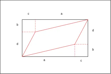
Therefore, a determinant of 0, where an inverse matrix does not exist, can also be interpreted as the transformation not preserving the area of the region. In dimensions higher than 3, it is similarly interpreted as a value that scales the volume of the region. A negative determinant value can be interpreted as a change in the orientation of the basis (i.e., a flip).
The fact that $det(M_1 M_2) = det(M_1) \cdot det(M_2)$ can be understood not just as a numerical property but as a consequence of a sequence of transformations. This formula means that the transformation $M_1M_2$ changes the area of the original span by a factor that is the product of the scaling factors of $M_1$ and $M_2$.
2.5. System of Linear Equations
$$ Ax = b $$
This type of system of linear equations can be examined in detail using the concepts of span and determinant.
$det(A) = 0$ (the span is reduced): The question becomes whether the vector b exists within the reduced span. If a 3D span is reduced to a plane in 3D, the equation will be about whether the vector b lies on that plane. In this case, it means the column space defined by the columns of matrix A is not of full rank. This brings to mind the definition of the null space: as the dimension of the span is reduced, the entire region from the original span that gets mapped to the origin becomes the null space. That is, the solution set for $Ax = 0$ is the null space.
$det(A) \neq 0$: This is a one-to-one transformation, and an inverse matrix exists, so a unique solution exists. The solution will be: $x = A^{-1}b$. Through the determinant, it's possible to geometrically interpret Cramer's rule, which can find the solution for a system of linear equations in the case of a square matrix. Let's look at the diagram below.
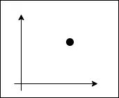
Let's call the point above $(x,y)$. The areas corresponding to the values of x and y can be drawn as follows:
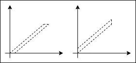
These are the region with area y formed by the vectors $(1,0)$ and $(x,y)$, and the region with area x formed by the vectors $(x,y)$ and $(0,1)$. If we apply a linear transformation through a matrix A to these regions, they will have new areas of $det(A) \cdot y$ and $det(A) \cdot x$ respectively (due to the property of the determinant). This corresponds to the area of the regions formed by $i'$ and $(x',y')$ and by $(x',y')$ and $j'$ respectively (see image below). Therefore, y and x represent the ratio of the areas when the transformed basis vectors $i'$ and $j'$ are replaced by the transformed vector for $(x,y)$.
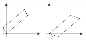
For example, given the following system of linear equations for a 2x2 square matrix:
$$ \begin{bmatrix} a & c \\ b & d \\ \end{bmatrix} \begin{bmatrix} x \\ y \\ \end{bmatrix} = \begin{bmatrix} \alpha \\ \beta \\ \end{bmatrix} $$
We can conveniently find the solution to this linear system by using the determinant values obtained by sequentially replacing each column with the solution vector $(\alpha, \beta)$. The method below is used computationally to find solutions to linear equations.
$$ y = \frac{ \det{\begin{bmatrix} a & \alpha \\ b & \beta \\ \end{bmatrix}} }{ \det{\begin{bmatrix} a & c \\ b & d \\ \end{bmatrix}} }, \quad x = \frac{ \det{\begin{bmatrix} \alpha & c \\ \beta & d \\ \end{bmatrix}} }{ \det{\begin{bmatrix} a & c \\ b & d \\ \end{bmatrix}} } $$
Even when the dimension is extended, the determinant is still defined as the amount by which volume is scaled, so solutions to linear equations in higher dimensions can be found in the same way. Also, when an inverse matrix does not exist, the determinant value is 0, making the denominator in the fraction 0, which similarly shows that no solution exists.
- continue to next post...