Link Copied!

Let's undertake a detailed mathematical and physical exploration, starting from Normalizing Flow, moving through Continuous Normalizing Flow and Conditional Flow Matching, and culminating in an understanding of why Rectified Flow adopts a Linear Path.
Due to its theoretical depth, easily accessible explanatory materials on Flow Matching are still scarce. It is challenging for many researchers and developers to gain a deep intuition for the fundamental question: 'Why are linear paths so effective?'. This article was written to address this gap by weaving the core ideas of Flow Matching—scattered across mathematics, physics, and recent papers—into a single, cohesive narrative, with the goal of providing an intuitive understanding of the 'Why' behind Flow Matching.

Introduction

The recent landscape of generative models can be broadly divided into two main approaches.

One is the Diffusion Model, which gradually generates an image from noise. The other is the Flow-based model, which directly connects noise and the image.

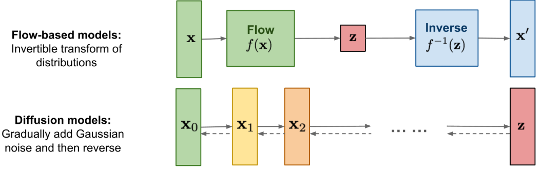
Diffusion Models, in particular, are based on a complex Stochastic Differential Equation (SDE). This method generates samples through a winding, unpredictable path, much like 'Brownian Motion,' where a particle moves about, buffeted by random forces. While this has shown outstanding performance, it inherently suffers from the drawback of slow generation speed due to the numerous steps required.

Against this backdrop, frameworks based on Ordinary Differential Equations (ODE) began to attract attention as an answer to the question, "Is there a faster, more efficient generation method?" Unlike SDEs, ODEs follow a deterministic path devoid of stochasticity. That is, once a starting point and an endpoint are determined, the path between them is uniquely and clearly defined.

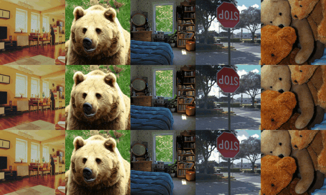
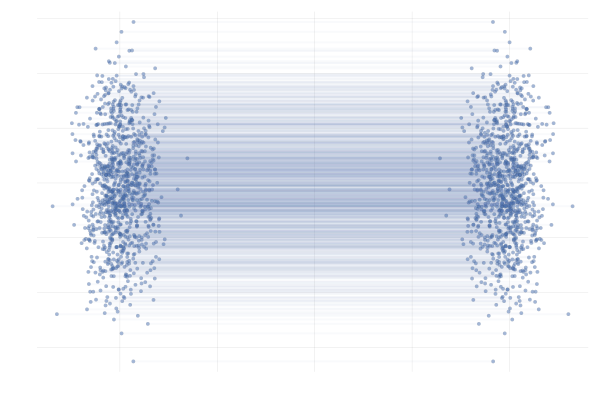
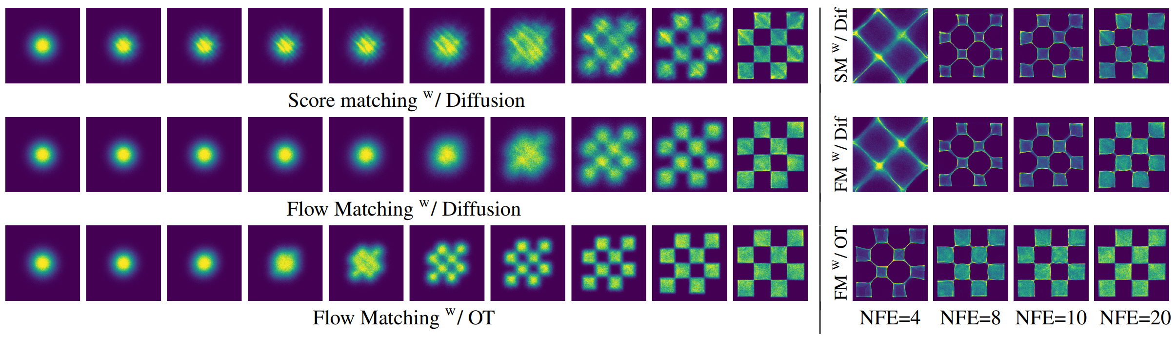
Top: Diffusion <-> Middle & Bottom: Flow-Matching. The difference between stochastic and deterministic paths is clearly visible.

Rectified Flow, built on this simple and powerful idea, has established itself as one of the most prominent state-of-the-art generative frameworks since its emergence. Rectified Flow assumes the simplest possible ODE path between noise $z_0$ and a target $z_1$: a straight line. This assumption stabilizes training and dramatically increases sampling speed.

In this article, we will first explore Flow Matching, which constitutes one pillar of these ODE-based generative models. We will then delve deep into Optimal Transport theory to uncover why one of its forms, Rectified Flow, adopted such a simple and powerful 'straight-line path'.

Part A. Flow Matching

1. Normalizing Flow

1.1. What is Flow

The idea behind flow-based models is simple and elegant.

"Can we learn a function that 'transforms' a simple, easy-to-handle probability distribution (e.g., a Gaussian distribution) into a complex, real-world data distribution that we want to approximate?"

The process of learning this 'transformation function' $\phi$ is called Normalizing Flow.

Input: A sample $x_0$ drawn from a noise distribution $p_0$.
Output: The result after passing through the transformation function, $x_1 = \phi(x_0)$.
Goal: To train $\phi$ such that the distribution of the output $x_1$ matches the real data distribution $p_1$, thereby generating plausible images.

Therefore, the learning objective is to find a continuous, differentiable, and invertible mapping function $\phi$ that satisfies the relationship: $$ \phi(x_0) = x_1 \sim p_1 $$

To achieve this goal, we need to calculate the probability that the transformed sample $x_1$ belongs to the data distribution $p_1$—that is, the likelihood $p_1(x_1)$—and maximize it.

1.2. Likelihood of Normalizing Flow

By applying the Change of Variables Theorem to express the relationship between $x_1$ and $x_0$, we obtain the principle that the infinitesimal probability (probability mass) must be conserved before and after the transformation $\phi$.

$$ p_1(x_1)|dx_1| = p_0(x_0)|dx_0| $$

Rearranging for $p_1(x_1)$ and using the relationship $x_0 = \phi^{-1}(x_1)$, we get the following:

$$ p_1(x_1) = p_0(\phi^{-1}(x_1)) \left| \det\left( \frac{\partial \phi^{-1}(x_1)}{\partial x_1} \right) \right| $$

A non-linear function $\phi^{-1}$ can be locally approximated by a linear transformation in the vicinity of $x_1$. The matrix representing this local linear transformation is the Jacobian $$ J_{\phi^{-1}}(x_1) = \frac{\partial \phi^{-1}(x_1)}{\partial x_1} $$
Here, $\det(\cdot)$ is a value that corrects for the change in the volume of space due to the transformation. This is because, in linear algebra, the extent to which a linear transformation changes the volume of a space is measured by the determinant of the matrix representing that transformation (cf: Geometric Meaning of the Determinant).

Taking the logarithm of both sides of this equation yields the log-likelihood, which we can use as a loss function to maximize.

$$ \log p_1(x_1) = \log p_0(\phi^{-1}(x_1)) + \log \left| \det\left( \frac{\partial \phi^{-1}(x_1)}{\partial x_1} \right) \right| $$

However, this approach faces two major hurdles:

Invertibility: The inverse function $\phi^{-1}$ of the transformation function $\phi$ must be computable.
Computational Cost: The cost of calculating the Jacobian determinant, $\mathcal{O}(D^3)$, is prohibitively expensive for high-dimensional data.

2. Continuous Normalizing Flow

2.1. Continuous Flow

To solve this problem, a new idea emerged:

"Instead of a single, massive transformation function $\phi$, what if we think of it as a 'Flow' connecting an infinite number of tiny changes?"

This means modeling the transformation process as a continuous trajectory over time.

On this trajectory, the sample $x_0$ is the position at time $t=0$, and the desired data $x_1$ is the final position at time $t=1$.

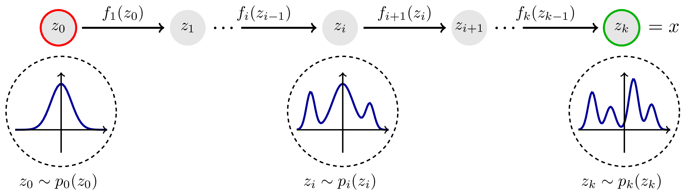
That is, the transformation $\phi$ is expressed as a composition of multiple functions, $$ \phi = \phi_{(T-1)\cdot \triangle t} \ \circ \dots \circ \phi_{1 \cdot \triangle t} \circ \phi_{0 \cdot \triangle t} $$ and the following relationship holds for each function: $$ \phi_t(x_t) = x_t + \triangle t \cdot u_t(x_t), \ \triangle t = \frac{1}{T} $$

Now, if we consider the limit as $$ T \rightarrow \infin $$ the change in the sample is no longer described by a single function but by an Ordinary Differential Equation (ODE).

$$ \frac{dx_t}{dt} = u_t(x_t) $$

Here, $u_t(x_t)$ is a velocity vector field that defines the direction and speed at which a 'particle' of probability density at a given position $x_t$ and time $t$ should move. Our goal now is to learn this velocity field $u_t$ with a neural network, instead of the transformation function $\phi$.

2.2. Likelihood of CNF

The most dramatic advantage of introducing a Continuous Flow is the fundamental change in how the likelihood is calculated. The Jacobian determinant, which was nearly impossible to compute in discrete transformations, is replaced by the much more manageable integral of the divergence.

To understand this principle, let's start by viewing probability as a 'fluid'.

2.2.1. Probability Fluid and Flow

Imagine a probability distribution $p_t(x)$ that changes over time.

This can be thought of as the density distribution of countless microscopic 'probability particles' spread throughout space (as particles move, the density in some areas will increase while it decreases in others). Let's first clarify a few terms from this perspective.

Probability Current:

The movement of these probability particles is described by the velocity vector field $u_t(x_t)$. However, velocity alone does not tell us the 'amount of flow'.
In a region where the density is zero, there are no particles flowing, no matter how high the velocity. It is natural to define the actual 'amount of probability flow' at a specific point $x$ as the product of the density $p_t(x)$ and the velocity $u_t(x)$. This is called the Probability Current $$ J_t(x) = p_t(x) u_t(x) $$ and this vector indicates the direction and magnitude of the probability flow at that point.

Net Outflow:

Consider an infinitesimal volume. The reason the probability density within this volume changes over time ($\partial p_t / \partial t$) is singular: probability has flowed in or out across its boundary.
The mathematical tool for expressing this 'difference between inflow and outflow', or net outflow, is the Divergence $\nabla$.
Divergence measures how much a vector field (in this case, the probability flow $J_t$) 'emanates from (source)' or 'disappears into (sink)' a specific point.
- $\nabla \cdot J_t > 0$: Probability is flowing out of the point (→ density decreases).
- $\nabla \cdot J_t < 0$: Probability is flowing into the point (→ density increases).
Mathematically, it is defined as the sum of the partial derivatives in each direction. $$ \nabla \cdot u_t = \frac{\partial u_1}{\partial x_1} + \frac{\partial u_2}{\partial x_2} + \dots + \frac{\partial u_D}{\partial x_D} = \sum_{i=1}^D \frac{\partial u_i}{\partial x_i} $$

Therefore, the rate of change of density at a point is equal to the net outflow with a negative sign. Expressing this as an equation gives us the Continuity Equation.

$$ \boxed{\frac{\partial p_t(x)}{\partial t} = - \nabla \cdot J_t(x) = - \nabla \cdot (p_t(x) u_t(x))} $$

This equation mathematically expresses the law of conservation of probability mass: "probability is neither created nor destroyed, and its density changes only through flow."

In addition to deterministic drift (ODE), a more general partial differential equation that considers random noise like Brownian motion is known as the Fokker-Planck Equation.

$$ \frac{\partial p_t(x)}{\partial t} = \underbrace{-\nabla \cdot [f(x,t)p_t(x)]}_{\text{Drift (flow)}} + \underbrace{\frac{1}{2}\sum_{i,j} \frac{\partial^2}{\partial x_i \partial x_j} [[g(t)g(t)^T]_{ij} p_t(x)]}_{\text{Diffusion}} $$

Since a Continuous Normalizing Flow (CNF) is a purely deterministic form with no diffusion term ($g=0$), the dynamics of the probability distribution followed by a CNF can be seen as a special case of the Fokker-Planck Equation, namely the Continuity Equation.

2.2.2. Derivation of Log-Likelihood

We now need to calculate the rate of change of the log probability that a particle experiences as it moves, i.e., $ \frac{d}{dt} \log p_t(x_t) $.

This can be expressed as the sum of two effects:

The effect of the distribution itself changing over time (Eulerian perspective): The change in density at my position even if I stay still ($x$ fixed) as time passes. $$ \frac{\partial}{\partial t} \log p_t $$
The effect of moving to a region of different density (Lagrangian perspective): The change in density because I move with velocity $u_t$ to a location with a different density. $$ \frac{dx_t}{dt} \cdot \nabla \log p_t $$

These two are combined in the Total Derivative: $$ \frac{d \log p_t(x_t)}{dt} = \frac{\partial \log p_t(x_t)}{\partial t} + \frac{dx_t}{dt} \cdot \nabla_x \log p_t(x_t) $$

Since ${dx_t}/{dt} = u_t(x_t)$, we get:

$$ \frac{d \log p_t(x_t)}{dt} = \frac{\partial \log p_t(x_t)}{\partial t} + u_t(x_t) \cdot \nabla_x \log p_t(x_t) \quad \cdots \text{(eqn. 1)} $$

i. First Term

Now let's look at the first term, $\partial \log p_t / \partial t$. We know that (from the chain rule for logarithms): $$\frac{\partial \log p_t}{\partial t} = \frac{1}{p_t} \frac{\partial p_t}{\partial t} $$

Do you see that $\partial p_t / \partial t$ is the continuity equation we discussed above? By substituting the continuity equation here, we get the relationship: $$\frac{\partial \log p_t}{\partial t} = -\frac{1}{p_t} \nabla \cdot (p_t u_t) $$

Now, after distributing the product rule for divergence as follows, $$\nabla \cdot (p_t u_t) = (\nabla p_t) \cdot u_t + p_t (\nabla \cdot u_t) $$ we can obtain the result below. $$\frac{\partial \log p_t}{\partial t} = -\frac{1}{p_t} [(\nabla p_t) \cdot u_t + p_t (\nabla \cdot u_t)] = - \left( \frac{1}{p_t} \nabla p_t \right) \cdot u_t - (\nabla \cdot u_t) $$

Using the relationship $\nabla \log p_t = \nabla p_t / p_t$ (the score function), the first term simplifies to: $$\frac{\partial \log p_t}{\partial t} = -(\nabla \log p_t) \cdot u_t - (\nabla \cdot u_t) \quad \cdots \text{(eqn. 2)} $$

ii. Final Equation

Finally, let's substitute the result we just obtained (eqn. 2) back into eqn. 1: $$ \frac{d \log p_t(x_t)}{dt} = \frac{\partial \log p_t(x_t)}{\partial t} + u_t(x_t) \cdot \nabla_x \log p_t(x_t) \quad \cdots \text{(eqn. 1)} $$

$$ \begin{aligned} \frac{d \log p_t(x_t)}{dt} &= \underbrace{\left[-(\nabla \log p_t) \cdot u_t - (\nabla \cdot u_t)\right]}_{\text{from (eqn. 2)}} + u_t \cdot \nabla \log p_t \\ &= - \nabla \cdot u_t(x_t) \end{aligned} $$

As a result, we have arrived at the following very concise final equation:

$$ \frac{d \log p_t(x_t)}{dt} = - \nabla \cdot u_t(x_t) $$

2.2.3. Divergence & Trace

The reason this result is revolutionary is that the divergence $\nabla \cdot u_t$ is equal to the trace of the Jacobian matrix of the velocity field $u_t$.

$$ \nabla \cdot u_t = \sum_{i=1}^D \frac{\partial u_{t,i}}{\partial x_i} = \text{Tr}\left( \frac{\partial u_t}{\partial x_t} \right) $$

This becomes self-evident if we re-examine the definitions of Divergence and the Jacobian.

Divergence: $$ \nabla \cdot u_t = \frac{\partial u_1}{\partial x_1} + \frac{\partial u_2}{\partial x_2} + \dots + \frac{\partial u_D}{\partial x_D} = \sum_{i=1}^D \frac{\partial u_i}{\partial x_i} $$
Jacobian:

$$ J_u = \frac{\partial u}{\partial x} = \begin{pmatrix} \frac{\partial u_1}{\partial x_1} & \frac{\partial u_1}{\partial x_2} & \cdots & \frac{\partial u_1}{\partial x_D} \\ \frac{\partial u_2}{\partial x_1} & \frac{\partial u_2}{\partial x_2} & \cdots & \frac{\partial u_2}{\partial x_D} \\ \vdots & \vdots & \ddots & \vdots \\ \frac{\partial u_D}{\partial x_1} & \frac{\partial u_D}{\partial x_2} & \cdots & \frac{\partial u_D}{\partial x_D} \end{pmatrix} $$

If we compute the trace of this Jacobian matrix, we find: $$ \text{Tr}(J_u) = \frac{\partial u_1}{\partial x_1} + \frac{\partial u_2}{\partial x_2} + \dots + \frac{\partial u_D}{\partial x_D} $$ which is identical to the definition of divergence.

This result is also intuitively obvious. If we consider the meaning of the off-diagonal elements (${\partial u_i}/{\partial x_j}$ , $i \neq j$), they represent how the velocity component in the $i$-th direction changes when moving in the $j$-th direction.

In other words, they induce rotation or shear, not a change in the fluid's volume (expansion/contraction). Since what we wanted to calculate with the determinant was the rate of change of volume under a linear transformation, it becomes clear that these off-diagonal elements do not contribute.

In conclusion, the Jacobian determinant calculation required for discrete transformations is replaced by the calculation of the Jacobian trace in continuous flows. The determinant depends on all elements and has a computational complexity of $\mathcal{O}(D^3)$, whereas the trace is simply the sum of the diagonal elements, making it much simpler to compute.

3. Flow Matching

While Continuous Normalizing Flow (CNF) facilitated computation by replacing the Jacobian determinant with the integral of the trace, a serious problem remained: slow training speed. To calculate the log-likelihood, the ODE had to be solved at every training step, which was essentially like repeating the slow sampling process of a diffusion model each time.

The ideal loss function for training a velocity field $v_\theta(x_t, t)$ with a Neural Network is as follows:

$$ \mathcal{L} = \mathbb{E}_{t \sim \mathcal{U}, x_t \sim p_t} [\|v_\theta(x_t, t) - u_t(x_t)\|^2] $$

This loss function is a regression problem that predicts the actual velocity field $u_t(x_t)$ at a point, given a sample $x_t$ at time $t$.

$v_\theta(x_t, t)$: The predicted velocity vector field from the network we are training.
$u_t(x_t)$: The 'ground truth' marginal vector field we need to know.

This is structurally similar to the ground truth noise regression problem in DDPM, but there is a crucial difference: the fact that "we do not know the 'ground truth' marginal velocity field $u_t(x_t)$ that transforms the entire data distribution $p_0$ to $p_1$."

This velocity field is a complex quantity representing the change of the entire data distribution $p_t(x)$ at time $t$, and it is impossible to compute directly.

3.1. Conditional Flow Matching

To break this impasse, a trick called Conditional Flow Matching (CFM) was introduced. The core idea of CFM can be summarized as follows:

"Instead of directly learning the complex 'marginal vector field' $u_t(x)$ that follows the path of the entire distribution $p_t(x)$, let's train the network to mimic a simple 'conditional vector field' $u_t(x|z_1)$ that connects individual sample pairs ($z_0$, $z_1$)."

Let's look at how this is possible, step by step.

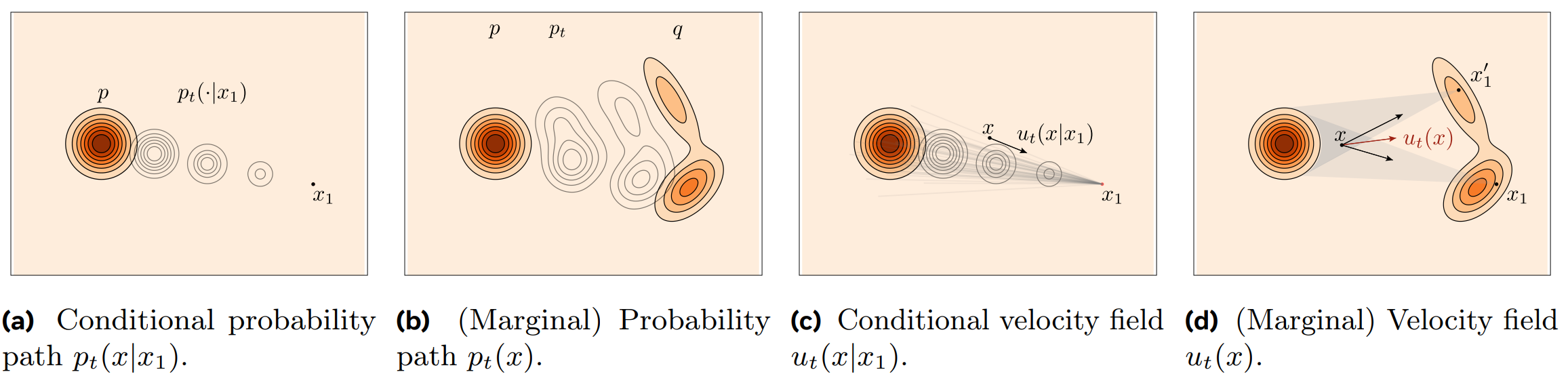
3.1.1. Conditional Probability Path

Instead of the unknown path $p_t(x)$ of the entire distribution, we can directly define a manageable Conditional Probability Path $p_t(x|x_1)$. This is the probability distribution of where a particle will be at time $t$, given a data sample $x_1$.

A representative method is to define the path as the trajectory of a Gaussian distribution: $$ p_t(x|x_1) = \mathcal{N}(x | \mu_t(x_1), \sigma_t^2(x_1)I) $$ We can set the boundary conditions such that at time $t=0$, it is a standard normal distribution (complete noise), and at time $t=1$, it reaches the target data $x_1$.

$t=0$: $\mu_0(x_1) = 0, \sigma_0(x_1) = 1$
$t=1$: $\mu_1(x_1) = x_1, \sigma_1(x_1) = \sigma_{min} \approx 0$

This has the exact same conceptual structure as the Forward Process $q(x_t|x_0)$ in diffusion. While DDPM defined a path from $x_0$ to noise, CFM can be interpreted as fixing the target $x_1$ and defining a virtual path towards it.

Now, from our self-designed path $p_t(x|x_1)$, we can also derive the conditional vector fields $u_t(x|x_1)$ that generate this path, via the continuity equation.

$$ {\frac{\partial p_t(x_t)}{\partial t} = - \nabla \cdot (p_t(x_t) u_t(x_t))} $$

From the continuity equation above, the following conditional vector fields are derived.

$$ {\frac{\partial p_t(x_t | x_1)}{\partial t} = - \nabla \cdot (p_{t|1}(x_t | x_1) u_t(x_t | x_1))} $$

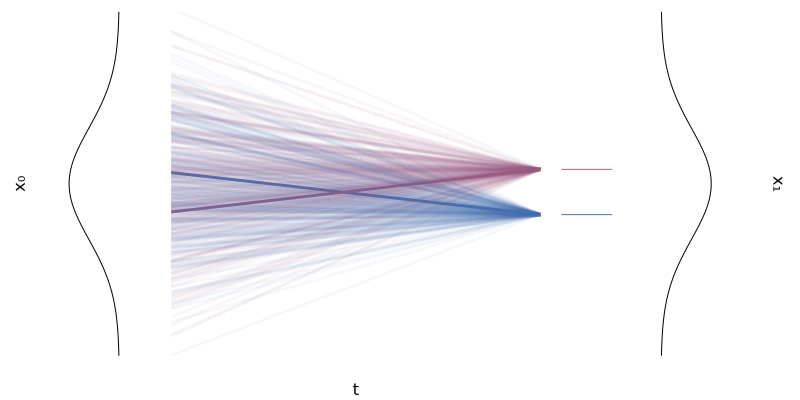
Remember that there are infinitely many conditional vector fields that satisfy a given conditional probability.

path 1	path 2

3.1.2. Conditional Flow Matching

Now let's examine two important mathematical facts at the core of CFM.

_ The marginal vector field is the expectation of the conditional vector fields._

The marginal vector field $u_t(x_t)$ can be expressed through the conditional vector fields $u_t(x_t|x_1)$ as follows (using Bayes' rule): $$ u_t(x_t) = \int u_t(x_t|x_1) \frac{p_{t|1}(x_t | x_1) p_1 (x_1)}{p_t(x_t)} dx_1 $$

And if we rearrange the continuity equation we saw earlier, $$ {\frac{\partial p_t(x_t | x_1)}{\partial t} = - \nabla \cdot (p_{t|1}(x_t | x_1) u_t(x_t | x_1))} $$ using Bayes' rule, we can see that the following holds.

$$ \begin{aligned} \frac{\partial p_t(x_t)}{\partial t} &= \boxed{\frac{\partial}{\partial t} \int p_{t|1}(x_t | x_1)} \ p_1 (x_1) dx_1 \\ &= \boxed{ - \int \nabla \cdot (p_{t|1}(x_t | x_1) u_t(x_t | x_1)) }\ p_1 (x_1) dx_1 \\ &= - \nabla \cdot \left ( \boxed{ \int u_t(x_t | x_1)) \frac{p_{t|1}(x_t | x_1) p_1 (x_1)}{p_t(x_t)} dx_1 } \ p_t(x_t) \right ) \\ &= - \nabla \cdot \bigg [ \boxed{u_t(x_t)} \ p_{t}(x_t ) \bigg ] \end{aligned} $$

In other words, the marginal vector field $u_t(x_t)$ at a point $x_t$ is equal to the average of all possible conditional vector fields $u_t(x_t|x_1)$ that pass through that point. $$ u_t(x_t) = \mathbb{E}_{p(x_1|x_t)}[u_t(x_t|x_1)] = \int u_t(x_t|x_1) p(x_1|x_t) dx_1 $$

_ Therefore, the total loss function is equivalent to the conditional loss function._

From the first fact, it is proven that the ideal but computationally infeasible loss function we wanted to solve is equivalent to the computable conditional loss function.

$$ \mathcal{L}_{\text{marginal}} = \mathbb{E}_{t, x_t} [\|v_\theta - u_t\|^2] \\ \iff \\ \mathcal{L}_{\text{CFM}} = \mathbb{E}_{t, x_1, x_t|x_1} [\|v_\theta - u_t(\cdot|x_1)\|^2] + C $$

The reason the two losses are equivalent becomes clear when we examine the inner product term that appears when expanding the loss function.

$$ \begin{aligned} \mathbb{E}_{x_t \sim p_t} [\langle v_\theta(x_t), u_t(x_t) \rangle] &= \int \left[ v_\theta(x_t) \cdot \boxed{u_t(x_t)} \ \right ]p_t(x_t) dx_t \\ &= \int \left[ v_\theta(x_t) \cdot \boxed{\int u_t(x_t|x_1) p_t(x_1|x_t) dx_1 } \right ]p_t(x_t) dx_t \\ &= \iint v_\theta(x_t) \cdot u_t(x_t|x_1) \boxed{ p_t(x_1|x_t) p_t(x_t)} dx_1 dx_t \\ &= \iint v_\theta(x_t) \cdot u_t(x_t|x_1) \boxed{p(x_1, x_t)} dx_1 dx_t \\ &= \mathbb{E}_{(x_1, x_t) \sim p(x_1, x_t)} [\langle v_\theta(x_t), u_t(x_t|x_1) \rangle] \end{aligned} $$

This means we can perfectly replace the regression problem for the unknown $u_t$ with a regression problem for $u_t(\cdot|x_1)$, which we have designed and for which we know the answer.

3.1.3. Sampling w/ Conditional Flow

Finally, let's consider how we sample the training data $x_t \sim p_t(x|x_1)$.

Instead of sampling directly from a Gaussian Distribution, CFM uses a more efficient Conditional Flow Map $\phi_t$.

$$ x_t = \phi_t(x_0|x_1) = \sigma_t(x_1)x_0 + \mu_t(x_1) $$

This is a function that deterministically maps a noise sample $x_0$ from a standard normal distribution (base distribution, $p_0$) to a point $x_t$ on the target distribution $p_t(x|x_1)$ at time $t$.

Thanks to this, we can generate the necessary training data $x_t$ with simple addition and multiplication, without needing to sample from complex distributions.

3.2. Final Training Algorithm

Combining all these processes, the final training algorithm becomes remarkably simple.

Sampling: Sample noise $x_0 \sim p_0$ from the base distribution and $x_1 \sim p_1$ from the real data distribution.
Time Sampling: Sample a time $t \sim \mathcal{U}$ uniformly.
Trajectory Path: Calculate a point on the path $x_t = \phi_t(x_0|x_1)$ using the Conditional Flow Map.
Target Velocity: Calculate the 'ground truth' velocity $u_t(x_t|x_0, x_1)$ for that path.
Training: Minimize the following loss to have the Neural Network $v_\theta(x_t, t)$ predict the target velocity: $ \mathcal{L} = |v_\theta(x_t, t) - u_t(x_t|x_0, x_1)|^2 $

In conclusion, Flow Matching completely eliminates the need to solve ODEs during training and transforms the problem into a simple regression task of predicting the slope of the path connecting two points.

This idea of a 'deterministic path connecting two points' aligns with the core insight of DDIM, and Flow Matching incorporates this into the learning paradigm itself, dramatically increasing the training efficiency of generative models.

3.3. Rectified Flow

Within the framework of CFM, we are free to design any 'Conditional Path'. Here, Rectified Flow makes the simplest and most intuitive choice.

"The simplest path connecting noise $x_0$ and data $x_1$ is a straight line."

This straight-line path is probabilistically expressed as $$ p_t(x_t|x_0, x_1) = \delta(x_t - ((1-t)x_0 + tx_1)) $$ and from a sampling perspective, it is as follows:

Path: $x_t = (1-t)x_0 + t x_1$
Velocity: The velocity required to create this path is a constant vector that depends only on the start and end of the path, i.e., $ u_t(x_t|x_0, x_1) = \frac{dx_t}{dt} = x_1 - x_0 $

Now, substituting this into the CFM loss function completes the final objective function for Rectified Flow.

$$ \mathcal{L} = \mathbb{E}_{t \sim U, x_0 \sim p_0, x_1 \sim p_1} \left[ \left\| v_\theta((1-t)x_0 + tx_1, t) - (x_1 - x_0) \right\|^2 \right] $$

The neural network learns to solve a very simple regression problem: given an intermediate point $x_t$, predict the direction vector from the start point to the destination ($x_1 - x_0$). This simplicity brings about dramatic improvements in training speed and stability.

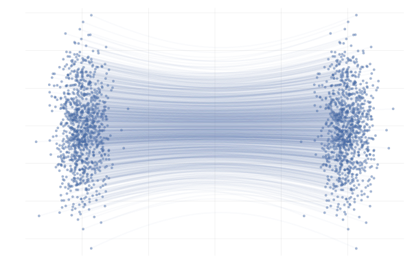
Finally, Rectified Flow has another advantage.

The coupling $(Z_0, Z_1)$ obtained from a single training run is already in a much more ordered (less entangled) state than the initial independent coupling $(X_0, X_1)$. What if we use this $(Z_0, Z_1)$ as new 'data' and train a Rectified Flow again? The Rectified Flow researchers showed that repeating this 'Reflow' process makes the travel paths of the samples exponentially closer to straight lines.

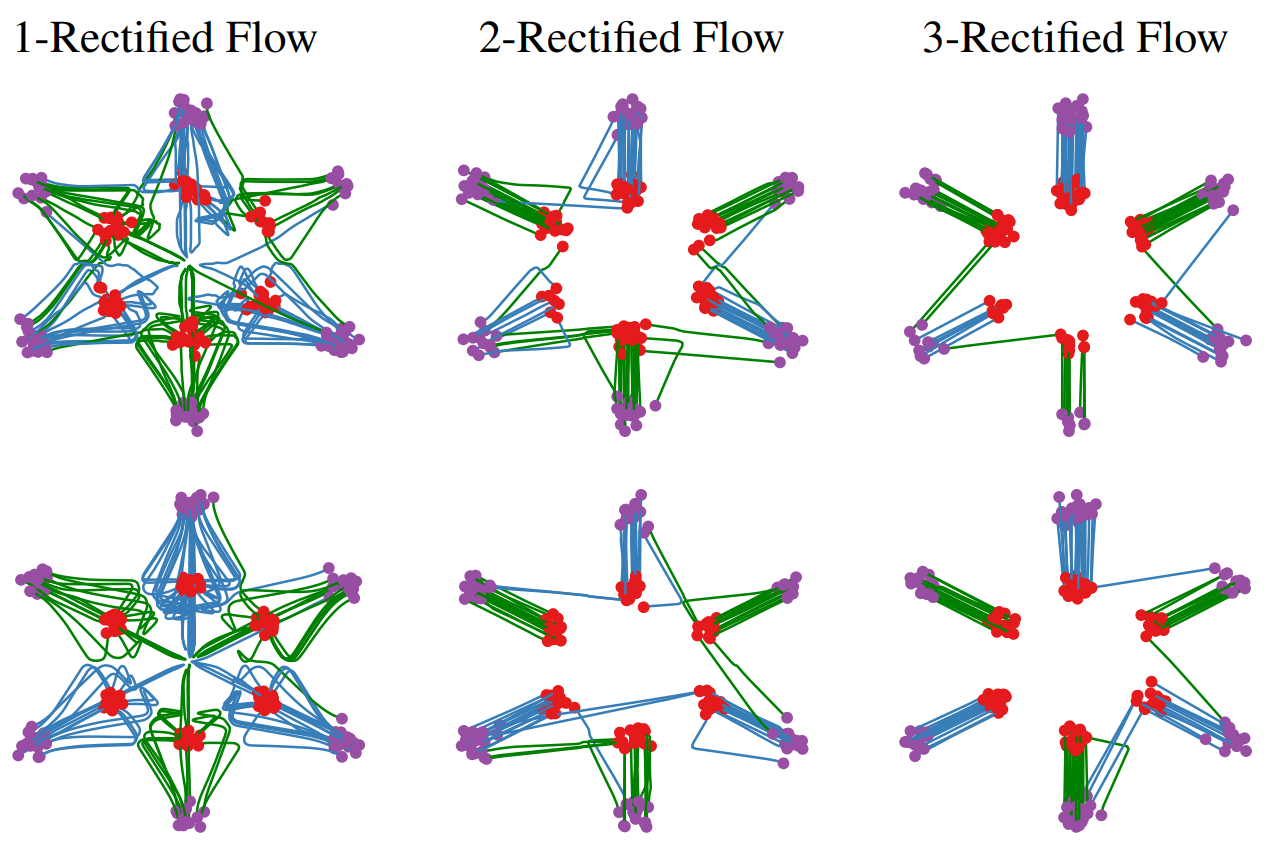
This means that a nearly perfect straight-line path can be learned with just a few iterations, which revolutionizes the number of ODE steps required during the generation process (even down to a single step), enabling very fast sampling.

Now we understand how we can learn a straight-line path through Flow Matching. But a fundamental question remains.

"Among the myriad possible paths, why is this 'straight' path so effective?"

Is it merely an engineering compromise for computational convenience? Or is there a deeper mathematical and physical principle hidden behind it?

Part B. Rectified Flow and Optimal Transport

To answer the preceding question, we will establish an assumption and explore the conclusions it leads to. The assumption is that the 'Cost' of a generative model finding a path from noise to data is equivalent to the 'Total Kinetic Energy' of particles moving in physics.

This is deeply related to the problem of Dynamic Optimal Transport, which minimizes the L2 Wasserstein distance between two distributions. To understand this, let's delve into the fundamental principles through the Least Action Principle of physics and the Optimal Transport theory of mathematics.

4. Optimal Transport

4.1. What is Optimal Transport

First, let's intuitively understand optimal transport. Imagine there's a hill of soil ($X$, the source distribution), and you need to dig up all this soil to fill a pit somewhere else ($Y$, the target distribution).

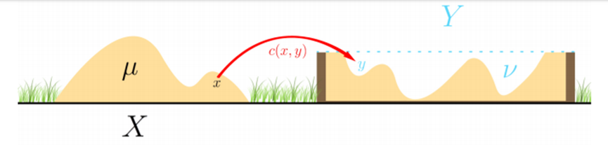
How should you move the soil to be "most efficient"?

'Efficient' means minimizing the total transportation cost. Optimal transport is the mathematical theory that finds this minimum-cost Transport Plan for converting one probability distribution (the pile of soil) into another (the pit).

4.2. Dynamic Optimal Transport

Traditional OT focuses on the final mapping—'which soil goes where'. However, in generative models, the path of the sample's gradual transformation is more important, which falls into the domain of Dynamic Optimal Transport. In Dynamic OT, we consider the change in distribution $p_t$ over time $t$ and the velocity field $v_t$ that creates this path.

To understand Rectified Flow's 'straight-line path' not as a simple mathematical trick but as a fundamental principle, it is necessary to understand the Principle of Least Action from physics.

5. Classical Mechanics

5.1. What is Action

In classical mechanics, when an object moves from one point to another, it chooses from among numerous possible paths the one that minimizes a physical quantity called Action, $S$. This is the Principle of Least Action.

This action is defined as the value of a quantity called the Lagrangian, $L$, integrated over time:

$$ S = \int_{t_0}^{t_1} L(x, \dot{x}, t) , dt $$

The Lagrangian $L$ is the kinetic energy ($T$) of the system minus its potential energy ($V$).

$$ L = T - V $$

The YouTube channel Veritasium has an excellent video explaining action, which I highly recommend: video link

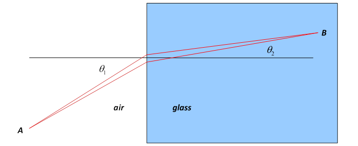
The phenomenon of light refraction, known as Fermat's Principle (minimizing time, not distance), is also an example of the Least Action Principle.

Now, let's consider the simplest case: a single particle moving in free space where no forces (like gravity or friction) are acting upon it. In this case, the potential energy is $V=0$, and the Lagrangian is purely kinetic energy.

$$ L = T = \frac{1}{2}m v^2 = \frac{1}{2}m ||\dot{x}||^2 $$

Since we are only interested in the mapping from one distribution to another and do not assume any external factors (Potential) that penalize specific paths, we can say that the cost of the system depends solely on the distance and velocity (Kinetic Energy) of the particles.

In this case, the action of this particle is:

$$ S = \int_{t_0}^{t_1} \frac{1}{2}m ||\dot{x}(t)||^2 , dt $$

According to the principle of least action, the particle moves along the path that minimizes this action $S$. Since the value inside the integral is always positive, the most intuitive way to minimize it would be to maintain a constant velocity ($||\dot{x}||$) and move along the shortest distance, i.e., a straight line.

Indeed, if we solve the differential equation to find the path that minimizes the above action, we find that the acceleration ($\ddot{x}$) is zero ($m\ddot{x} = 0$). This signifies uniform linear motion.

5.2. Euler-Lagrange Equation

The Euler-Lagrange Equation is a differential equation for the condition that makes the action minimal (or stationary, i.e., an extremum or a saddle point!).

It can be derived using the calculus of variations and is defined as follows: $$ \frac{\partial L}{\partial x} - \frac{d}{dt}\left(\frac{\partial L}{\partial \dot{x}}\right) = 0 $$

The meaning of each term in this equation is as follows:

${\partial L}/{\partial x}$: How much does the Lagrangian (cost) change when the position ($x$) of the path changes?
${\partial L}/{\partial \dot{x}}$: How much does the Lagrangian (cost) change when the velocity ($\dot{x}$) of the path changes? (Note: this value is equal to the momentum $p=mv$)
${d}/{dt}(\dots)$: How does the rate of change vary over time?

In other words, by solving the above equation, we can find the solution to the condition that minimizes the action. Now let's substitute the Lagrangian $L = \frac{1}{2}m\dot{x}^2$ we found in step 1 into this equation and calculate.

First Term: Calculating ${\partial L}/{\partial x}$

Let's look at the Lagrangian $L = \frac{1}{2}m\dot{x}^2$. This expression contains no position variable $x$; it only contains the velocity $\dot{x}$. Therefore, differentiating with respect to position $x$ gives a value of 0.

$$ \frac{\partial L}{\partial x} = \frac{\partial}{\partial x}\left(\frac{1}{2}m\dot{x}^2\right) = 0 $$

Intuitively, in free space, the cost (Lagrangian) is the same regardless of where the particle is. The cost only depends on how fast it is moving.

Second Term: Calculating $\frac{d}{dt}\left(\frac{\partial L}{\partial \dot{x}}\right)$ First, let's look at ${\partial L}/{\partial \dot{x}}$. Differentiating the Lagrangian $L = \frac{1}{2}m\dot{x}^2$ with respect to velocity $\dot{x}$, we get:

$$ \frac{\partial L}{\partial \dot{x}} = \frac{\partial}{\partial \dot{x}}\left(\frac{1}{2}m\dot{x}^2\right) = \frac{1}{2}m(2\dot{x}) = m\dot{x} $$

Now, differentiating this result with respect to time $t$:

$$ \frac{d}{dt}\left(m\dot{x}\right) $$

Since mass $m$ is a constant, it comes out of the derivative, and differentiating velocity $\dot{x}$ with respect to time gives acceleration $\ddot{x}$.

$$ \frac{d}{dt}\left(m\dot{x}\right) = m \ddot{x} $$

Now, substituting the two results back into the equation: $$ \frac{\partial L}{\partial x} - \frac{d}{dt}\left(\frac{\partial L}{\partial \dot{x}}\right) = 0 $$ $$ 0 - m\ddot{x} = 0 $$ Since the mass $m$ is not 0, for this equation to hold, the following condition must be met:

$$ \ddot{x} = 0 $$

This means the acceleration is 0, signifying uniform linear motion.

5.3. Action in Optimal Transport

5.3.1. Action in Probability Distribution

Now let's extend this concept from a single particle to a collection of countless particles, i.e., a probability distribution.

Kinetic Energy of a Single Particle: $T = \frac{1}{2}m ||v||^2$
Total Kinetic Energy of a Probability Distribution: The expected value of the kinetic energies of all particles constituting the distribution.

Let the distribution at time $t$ be $p_t(x)$, and the velocity of particles at each point $x$ be represented by the velocity field $v_t(x)$. The total kinetic energy at a specific time $t$ can be calculated by taking a weighted average of the kinetic energy at each point ($\frac{1}{2}||v_t(x)||^2$) by the density at that point ($p_t(x)$).

$$ \text{Total Kinetic Energy at } t = \mathbb{E}_{x \sim p_t}\left[\frac{1}{2}||v_t(x)||^2\right] = \int \frac{1}{2}||v_t(x)||^2 p_t(x) ,dx $$

Just like a free particle, if we assume a transformation of a distribution with no external forces (i.e., no potential energy), the Lagrangian of this system becomes its total kinetic energy. Therefore, the action of the entire transformation process is the integral of this total kinetic energy over time.

$$ \mathcal{A}(p_t, v_t) = \int_0^1 \left( \int \frac{1}{2}||v_t(x)||^2 p_t(x) ,dx \right) dt $$

As with the principle of least action, we seek to find the path ($p_t, v_t$) that minimizes this action.

This redefinition of the transformation of a probability distribution as a problem of finding a path that minimizes total kinetic energy (Action) corresponds exactly to the core idea of the 'Benamou-Brenier formula' in optimal transport, a formulation of dynamic OT. We are, in essence, solving a problem of generative models in the language of fluid dynamics.

5.3.2. Constrained Euler-Lagrange Equation

There is one constraint here. Do you remember the continuity equation from the Flow section? It was an equation representing the conservation of probability mass, stating that particles (probability mass) are neither created nor destroyed.

Since we are solving a problem for a probability distribution, the continuity equation becomes the constraint we must adhere to.

$$ \frac{\partial p_t}{\partial t} =- \nabla \cdot (p_t v_t) $$

To solve such a constrained optimization problem, we introduce a Lagrange Multiplier function $\phi(x, t)$. This function combines the constraint with the action to create a new functional $\mathcal{L}$.

$$ \mathcal{L}[p, v, \phi] = \mathcal{A}[p, v] - \int_0^1 \int_{\mathbb{R}^d} \phi(x, t) \left( \frac{\partial p_t}{\partial t} + \nabla \cdot (p_t v_t) \right) ,dx ,dt $$

Now we can transform the problem into optimizing the unconstrained functional $\mathcal{L}$. On the optimal path, $\mathcal{L}$ must be stable with respect to infinitesimal variations in $p$, $v$, and $\phi$. That is, the functional derivative with respect to each variable must be zero.

To facilitate calculation, let's apply integration by parts to the constraint term to move the derivatives from $p$ and $v$ to $\phi$.

$$ \mathcal{L} = \int_0^1 \int_{\mathbb{R}^d} \left( \frac{1}{2} |v|^2 p + p \frac{\partial \phi}{\partial t} + p v \cdot \nabla \phi \right) dx dt - \int_{\mathbb{R}^d} [\phi p]_0^1 dx $$

Now, we use this expression to calculate the variation for each variable.

Functional derivative with respect to Velocity $v$ We take the functional derivative of $\mathcal{L}$ with respect to velocity $v$ ($\delta_v \mathcal{L}$) and set the result to 0.

Differentiating the integrand with respect to $v$ gives $p v + p \nabla \phi = p(v + \nabla \phi)$, and for this value to be 0, the following must hold: $$ v + \nabla \phi = 0 $$

Thus, we obtain the first key result: the optimal vector field ($v_t$) must be the gradient of some scalar potential function ($\phi$). $$ {v_t(x) = -\nabla \phi(x, t)} $$

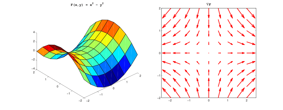- Vector field (right) and corresponding scalar potential (left).

Functional derivative with respect to Density $p$

Now, we take the functional derivative of $\mathcal{L}$ with respect to density $p$ ($\delta_p \mathcal{L}$) and set the result to 0. The integrand is linear in $p$, so for this variation to be 0, the term in the parentheses must be 0. $$ \frac{1}{2} |v|^2 + \frac{\partial \phi}{\partial t} + v \cdot \nabla \phi = 0 $$

Hamilton-Jacobi Equation Now, let's substitute the first result ($v = -\nabla \phi$) into the second result. $$ \frac{1}{2} |-\nabla \phi|^2 + \frac{\partial \phi}{\partial t} + (-\nabla \phi) \cdot (\nabla \phi) = 0 $$

$$ \frac{1}{2} |\nabla \phi|^2 + \frac{\partial \phi}{\partial t} - |\nabla \phi|^2 = 0 $$

Simplifying this, we obtain the partial differential equation that the potential function $\phi$ must satisfy, which is the Hamilton-Jacobi Equation. $$ {\frac{\partial \phi}{\partial t} - \frac{1}{2} |\nabla \phi(x, t)|^2 = 0} $$

This equation is a fundamental equation in classical mechanics that describes the motion of a free particle.

Proving that acceleration is 0 Finally, let's consider the path $x(t)$ of a particle moving along this optimal vector field. The particle's velocity is $\dot{x}(t) = v_t(x(t))$. We need to show that the acceleration of this particle, $\ddot{x}(t)$, is 0.

The acceleration $\ddot{x}(t)$ is the total derivative of the velocity $v_t(x(t))$ with respect to time. $$ \ddot{x} = \frac{d}{dt} v_t(x(t)) = \frac{\partial v}{\partial t} + (v \cdot \nabla)v $$ Let's express each term using the potential $\phi$.

First term: Using the derived Hamilton-Jacobi Equation ($\frac{\partial \phi}{\partial t} = \frac{1}{2}|v|^2$) and the relation $v = -\nabla\phi$, $$ \frac{\partial v}{\partial t} = \frac{\partial}{\partial t}(-\nabla \phi) = -\nabla\left(\frac{\partial \phi}{\partial t}\right) = -\frac{1}{2}\nabla(|v|^2) $$
Second term: Since the vector field $v$ is the gradient of a scalar potential $\phi$ ($v = -\nabla\phi$), its curl is zero ($\nabla \times v = \nabla \times (-\nabla\phi) = 0$). Therefore, $$ (v \cdot \nabla)v = \frac{1}{2}\nabla(|v|^2) $$ Now, combining the two terms to calculate the acceleration, $$ \ddot{x} = \frac{\partial v}{\partial t} + (v \cdot \nabla)v = -\frac{1}{2}\nabla(|v|^2) + \frac{1}{2}\nabla(|v|^2) = 0 $$

cf: $$\frac{1}{2}\nabla(A \cdot A) = (A \cdot \nabla)A + A \times (\nabla \times A) $$

5.4. Why is Rectified Flow Linear?

$$ \ddot{x}(t) = 0 $$

The acceleration of all particles following the optimal flow that minimizes the action and satisfies the continuity equation is zero. This mathematically proves that each particle undergoes uniform linear motion from its starting point $z_0$ to its destination $z_1$.

This is the strong theoretical background for why Rectified Flow takes the straight-line path connecting samples $z_0, z_1$ from two distributions as its learning target. The velocity vector $$v = z_1 - z_0$$ that the model learns corresponds to the velocity field of this optimal path.

Therefore, the 'straight-line path' $z_t = (1-t)z_0 + t z_1$ adopted by Rectified Flow is not an arbitrary choice but can be interpreted as the most natural and efficient path based on physical laws and mathematical optimization.

6. Rectified Flow on Manifold

In Part B, we showed through the principle of least action that the 'straight-line path' of Rectified Flow is the physically optimal path. The conclusion that the path minimizing Action in free space is uniform linear motion is clear and elegant.

However, one question remains.

"Does the data we handle truly live in 'free space'?"

It is much more reasonable to assume that high-dimensional data such as images, audio, and protein structures exist not in a simple Euclidean Space ($\mathbb{R}^d$), but on a complexly curved Manifold within it. A Manifold is a topology that locally has the properties of a Euclidean Space (a plane) (the reason flat-earthers think the Earth is flat!).

From this perspective, the conclusion of Part B has a critical limitation. The 'straight-line path' we derived is optimal only when assuming the space is flat. Just as the shortest path between two cities on the Earth's surface is not a straight line through the air but a curve along the surface (a great-circle route), the optimal path on a Manifold will no longer be a straight line.

So, has the idea of a 'straight line' in Rectified Flow hit a fundamental limit? To answer this question, we must extend the tools we built in Parts A and B from a flat Euclidean Space to a curved Riemannian Manifold.

A Riemannian Manifold $(M, g)$ consists of a space $M$ where each point $x$ locally looks like a Euclidean Space, and a Riemannian Metric $g$ that measures distances and angles on the Tangent Space $T_M$ at each point.

Now let's see how our key equations change on this curved space.

6.1. Dynamics on a Manifold

In Part A, we saw that the dynamics of a probability distribution are described by the Continuity Equation.

Euclidean Space: $${\frac{\partial p_t(x)}{\partial t} = - \nabla \cdot (p_t(x) u_t(x))}$$

This equation remains almost identical on a Manifold, with the Euclidean divergence ∇· simply being replaced by the Riemannian divergence div_g.

Riemannian Manifold: $${\frac{\partial p_t(x)}{\partial t} + \text{div}_g(p_t u_t)(x) = 0}$$

Thanks to this Riemannian continuity equation, one of the most important results we derived in Part A, the rate of change of the log-likelihood, also holds on a Manifold.

$$ \frac{d}{dt} \log p_t(\psi_t(x)) = - \text{div}_g(u_t)(\psi_t(x)) $$

This means that the core mechanism of Continuous Normalizing Flow remains valid even if the geometric structure of the data is not a Euclidean Space. We can still calculate the log-likelihood through the divergence of the velocity field u.

6.2. Flow Matching on a Manifold

Now we need to redefine the Loss function, our matching target.

In Euclidean Space, we measured the difference between two vectors using the L2 norm. On a Manifold, this role is taken over by the inner product $⟨·,·⟩_g$ defined by the Riemannian Metric $g$.

Therefore, the Loss function for Riemannian Conditional Flow Matching (RCFM) is as follows.

$$ \mathcal{L}_{\text{RCFM}}(\theta) = \mathbb{E}_{t, x_1, x_t|x_1} \left[ \left\| u_t(x_t|x_1) - v_\theta(x_t, t) \right\|^2_g \right] $$

Here, $||·||^2_g$ is the squared norm induced by the metric $g$, which measures the difference between two velocity vectors $u$ and $v$ when they exist in the same tangent space $T_{x_t}M$.

The key answer to the question about the L2 norm lies right here. The L2 norm is just a special case where the Riemannian Metric $g$ is the Euclidean metric, and the Flow Matching framework can accommodate any metric $g$ that better reflects the geometric structure of the data.

6.3. Geodesic Flow

The final question is this: What replaces the 'straight-line path' of Euclidean Space on a Manifold? The answer is the Geodesic, the shortest path connecting two points on a curved space (the shortest flight path for an airplane is also a geodesic).

Let's break down the linear interpolation of Rectified Flow once more. $$ x_t = (1-t)x_0 + t x_1 = x_0 + t(x_1 - x_0) $$ This simple equation actually hides three key actions.

Start at $x_0$
Follow the Direction $(x_1 - x_0)$
Move by $x_0 + t \cdot (x_1 - x_0)$

The key here is that "addition of a point and a vector" (+) and "subtraction of points" (-) are defined so naturally. This is because the space is flat, so the concepts of direction and distance are the same everywhere.

Now, let's bring this concept to a curved space, a Manifold. Taking our example of the Earth as a Manifold, if we think of 'starting point: Seoul' and 'destination: New York', then:

Direction: What does "New York's coordinates - Seoul's coordinates" mean? No matter what coordinate system you use (Spherical or Euclidean coordinates for latitude and longitude, what else!), it does not represent a direction vector. In a Manifold space, there is no simple way to obtain a direction vector by subtracting coordinates.
Move: Let's say we somehow obtained a direction vector. How do we travel from Seoul to New York? Where does Seoul's coordinates + travel distance * direction vector point to? In a Manifold, the 'addition' of a flat Euclidean space does not work.

In a curved space, we need to newly define "where to go" and "how to actually go in that direction". And what defines this is the Exponential Map.

Logarithmic Map: This calculates the 'initial velocity vector' $v \in T_{x_0}M$ of the shortest path from a starting point $x_0$ to a destination point $x_1$. This role is played by the Logarithmic Map. $$ v = \text{log}_{x_0}(x_1) $$
Exponential Map: This calculates the destination point when moving from a starting point $x_0$ with a velocity vector $v$ along a geodesic path for a duration $t$. This role is played by the Exponential Map. $$ x_t = \text{exp}_{x_0}(t \cdot v) $$

cf. The names Exp / Log here are not the exp, log operations we perform on scalar functions, but are closer in name to 'exp' as the solution to a linear differential equation, and 'log' as its inverse (the same concept as the exp/log map used between Lie Groups and Algebras). It is better to interpret them as generalized definitions of 'subtraction' and 'addition' on a Manifold.

Combining these two, we complete the Geodesic Conditional Flow on a Manifold.

$$ \psi_t(x_0|x_1) = \text{exp}_{x_0} (t \cdot \text{log}_{x_0}(x_1)) $$

This is the true meaning of Rectified Flow. The model is now trained to flow along the Geodesic, the shortest path on the Manifold, not a straight line in Euclidean space.

Now, if we redefine the Action of a free particle on a Manifold, the total kinetic energy is calculated using the Riemannian Metric $g$ and integrated over time. And the path that minimizes this Action is, by definition, the Geodesic.

Therefore, the 'straight-line path' idea of Rectified Flow was not a special case limited to Euclidean space. It reflects a deeper and more general physical principle of "following the path of least energy consumption (Action) under a given geometric structure (Manifold, metric)". The simple equation $$\ddot{x}=0$$ is replaced by the more complex geodesic equation on a Manifold, but the fundamental principle remains the same.

7. Last Discussion: Why Linear?

Q. The Mystery of Rectified Flow: Why Does the 'Wrong' Straight Path Work?

As we've seen, the most ideal transformation path we seek is the Geodesic, the shortest distance on a manifold. This generalizes the addition/subtraction of Euclidean space into the language of manifolds, exp/log maps, and can be considered the 'ultimate' form of Rectified Flow.

$$ \psi_t(x_0|x_1) = \exp_{x_0}(t \cdot \log_{x_0}(x_1)) $$

However, this beautiful theory hits the wall of computational infeasibility when faced with high-dimensional image data. Actual Rectified Flow models ignore all this complexity and use the simplest straight-line path, assuming the data space is flat.

$$ x_t = (1-t)x_0 + t x_1 $$

This path inevitably traverses the 'empty space' outside the low-dimensional manifold where the data exists. Although theoretically a 'wrong' path, this 'beautiful bias' works surprisingly well.

Why on earth is that?

1. Vector Field as a Corrective "Gravity Well"

Rectified Flow doesn't just learn a line connecting two points; it learns a Vector Field $v_\theta(x, t)$ defined over the entire space. The true mission of this vector field is as follows:

"If a particle $x_t$ is located in the 'empty space' off the manifold, provide the 'average optimal direction' to guide it back to the high-density region where data exists (the manifold)."

Mathematically, this is expressed as a Conditional Expectation. The model learns the average velocity over numerous data pairs $(X_0, X_1)$. $$ v_\theta(x_t, t) \approx \mathbb{E}[X_1 - X_0 \mid (1-t)X_0 + tX_1 = x_t] $$ If we reconsider this 'averaging' process, if a point $x_t$ is far from the manifold, the average direction of the numerous straight-line paths passing through it will naturally point towards the center of the manifold. It's as if a massive object (the data manifold) warps the surrounding space, creating a 'gravitational field'.

Therefore, when an ODE solver takes steps following this vector field, its actual trajectory is not a straight line but a smooth curve that follows the curvature of the manifold.

2. Implicit Space Straightening by Neural Networks

Powerful Deep Neural Networks like the Transformer do not process the input $x_t$ as is. The model is actually performing two tasks simultaneously.

Encoding (Unfolding): The initial layers of the network implicitly encode the complexly curved data manifold into an 'almost flat' latent feature space where linear operations are much more effective.
Decoding (Folding): The model predicts a simple direction vector in this 'straightened' space and then, through its later layers, 'decodes' that result back into a vector field suitable for the original curved space.

In other words, the model doesn't learn "how to forcibly follow a straight line in a curved space," but rather learns the "transformation itself that straightens the space, follows a straight line, and then reverts back to the original."

3. Starting in an Explicitly Straightened Latent Space

This idea is maximized in practical applications by recent models like the Latent Diffusion Model (LDM) and Stable Diffusion 3. These models learn the Flow not directly in pixel space, but within a well-trained VAE Latent Space.

The VAE latent space is designed to compress images into a semantically rich and structured space. In this space, the transformation between a 'cat photo' and a 'dog photo' is much more likely to have a linear and smooth path than in pixel space.

Therefore, our assumption changes from the strong one that "the million-dimensional image space is flat" to the much weaker and more reasonable assumption that "the thousand-dimensional 'space of concepts' learned by the VAE is (relatively) flat." This is one of the most practical reasons why Rectified Flow achieves such surprising performance.

In Closing

Thank you for reading this long article.

This piece actually began as a section explaining the Model Structure in a series I'm currently writing: Building a Large 3D Generative Model from Scratch.

Since Flow is a dominant framework for training networks not just for images and video, but also for 3D generation recently, I felt the need to clearly organize the fundamentals of flow. That section grew too long, so I decided to separate it into its own article.

I have tried to organize the content on flow to the best of my knowledge, but as my major is not in mathematics or physics, there may be errors in the process of developing concepts like action. I welcome any sharp corrections and teachings in the comments, and I will gratefully learn and revise accordingly.

Starting with the next article, I will return to the Building a Large 3D Generative Model from Scratch series and, as promised, delve into training in a multi-node environment. While the blog tends to focus more on understanding and explaining theory, this will be an uncharacteristically CS-focused post.

Thank you :)