Building Large 3D Generative Model (2) VAE and DiT Deep Dive

Link Copied!

Introduction

In the previous article, as the first step toward building a large 3D generative model, we took a deep dive into preparing the dataset and the essential data preprocessing pipeline, covering everything from mathematical and topological principles to actual algorithm implementation.

In this article, we will dissect the architecture of the Shape Generative Model, which lies at the very core of the 3D Generative Pipeline.

As briefly touched upon in previous posts, we will explore in detail the two different approaches within VAEs, from the VAE itself to the final generative model:

vecset-based
sparse voxel

C. VAE Architecture

There are two primary methods for compressing 3D data using a VAE. This choice goes beyond a mere implementation difference; it reflects a fundamental divergence in perspective on how to interpret 3D data.

Vecset-based VAE: Regards a 3D shape as an 'unordered set of points'.
Sparse Voxel VAE: Regards a 3D shape as a '3D grid with spatial structure'.

Let's compare and analyze how these two approaches lead to different architectures.

C.1. VecSet VAE

TLDR: From Mesh to an Unordered Set of Tokens

As the name suggests, the vecset-based VAE treats a 3D mesh as a set of vectors, specifically a PointCloud. This method was devised to naturally handle the challenges of 1) the variable number of vertices in a mesh and 2) the need for Rotation/Translation Invariance.

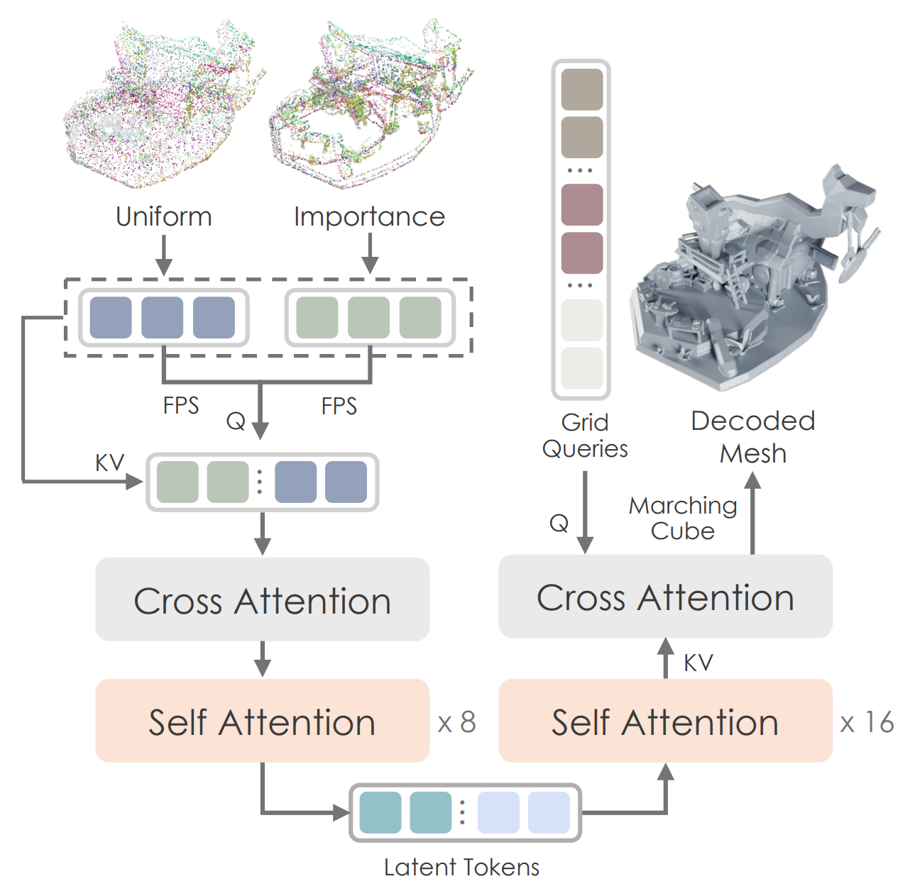
Figure: Hunyuan 3D 2.0's VAE. This showcases a vecset-based VAE architecture where sampled point clouds undergo Fourier featuring and are then passed through a Transformer Encoder/Decoder to predict an isosurface (SDF).

The latent encoding/decoding process of a Vecset-based VAE is relatively straightforward:

Surface Point Sampling: A fixed number of points (e.g., 4096) are sampled from the surface of a watertight mesh.
Fourier Feature Encoding: Positional Encoding (Fourier featuring) is applied to the 3D coordinates ($x, y, z$) of each sampled point. This encourages the model to focus on the relative positional relationships between points rather than absolute coordinates, thereby stabilizing the training process.
Transformer Encoder: The point vector sequence with applied Fourier features is passed through Transformer blocks to capture the global relationships between points, ultimately predicting a latent vector.

The core of this method is the conversion of the 3D structure into a 'Token Sequence' at the input data stage. The VAE's output, the latent vector, also takes the form of a 'tokenized' set of points with the shape [Batch, Num_points, Latent_dim]. This means that the subsequent generative model can directly receive the data without any separate preprocessing (like patchifying).

Now, let's take a detailed look at how this process is implemented in actual code.

1. Encoder: PointCloud to Latent Vector

The goal of the Encoder is to compress the point cloud into a fixed-size feature vector sequence that the VAE can handle.

First, after applying Fourier featuring to the 3D coordinates (x,y,z), instead of processing all points at once, a small number of representative points (pointcloud_query) extracted via Farthest Point Sampling (FPS) are used as Queries. The entire set of points serves as the Keys/Values for Cross-Attention. This can be interpreted as asking the model to "summarize the entire shape from the perspective of these representative points," enabling efficient information compression.

# vae/model.py : encode()

# ... FPS ...
fps_indices = data["fps_indices"]
pointcloud_query = torch.gather(pointcloud, 1, fps_indices.unsqueeze(-1).expand(-1, -1, pointcloud.shape[-1]))

# Perceiver: Cross-Attention
hidden_states = self.perceiver(pointcloud_query, pointcloud)

# Encoder: Self-Attention
for block in self.encoder:
    hidden_states = block(hidden_states)

The features that pass through the Perceiver then go through multiple layers of Self-Attention blocks, exchanging information among themselves and ultimately learning high-level relationships about the 3D shape.

2. Bottleneck

The reason a VAE can go beyond a simple autoencoder and enable sampling → generation in Generative AI lies in the ‘Reparameterization trick’ implemented through the DiagonalGaussianDistribution class in the bottleneck layer.

# vae/utils.py

class DiagonalGaussianDistribution:
    def __init__(self, mean, logvar, deterministic=False):
        self.mean, self.logvar = mean, logvar
        self.std = torch.exp(0.5 * self.logvar)
        # ...

    def sample(self, weight: float = 1.0):
        # Reparameterization Trick
        sample = weight * torch.randn(self.mean.shape, device=self.mean.device)
        x = self.mean + self.std * sample
        return x

The feature vector (latent vector) output by the Encoder is converted into a mean and log variance (logvar), which define the latent space. In __init__, these values define the mean and variance, i.e., the 'position' and 'degree of uncertainty' within the latent space.

The key here is the Reparameterization Trick implemented in the sample() method (drawing noise from a Gaussian distribution and using the mean and std to generate unnormalized noise). Thanks to this technique, backpropagation is possible across the entire model, even though it includes a non-differentiable 'sampling' process. $ \epsilon ' = \mu + \sigma \cdot \epsilon, \quad \epsilon \sim N(0, I) $

3. Decoder: Latent Vector to SDF

The Decoder's objective is to create a "continuous function" from the compressed latent vector, a function that can provide the SDF value for any arbitrary 3D coordinate we query.

# vae/model.py : decode() & query()

def decode(self, latent: torch.Tensor):
    hidden_states = self.proj_up(latent)
    for block in self.decoder:
        hidden_states = block(hidden_states)
    return hidden_states

def query(self, query_points: torch.Tensor, hidden_states: torch.Tensor):
    # query_points: 3D coordinates
    query_points = self.fourier_encoding(query_points)
    query_points = self.proj_query(query_points)

    query_output = self.attn_query(query_points, hidden_states)
    pred = self.proj_out(query_output)
    return pred

The decode() function uses the latent vector to perform Cross-Attention with the 3D coordinates for which we want to know the SDF values (query_points), ultimately predicting the final SDF value.

An important point to note is that the Vecset-based VAE approach carries the fundamental burden of having to solve two difficult problems simultaneously: (Compression + Modality Conversion).

Compression: Compressing the PointCloud, which represents the original mesh, into a low-resolution latent vector.
Modality Conversion: Generating a continuous 3D SDF from a discrete point cloud.

The problems that arise during this process are as follows:

Sampling Error: When sampling the PointCloud at the input stage, high-frequency details of the original mesh (like sharp edges or complex curved surfaces) are permanently lost.
Ill-posed Problem: The Decoder must infer the "empty space" between the sampled points. This is an ill-posed problem for which there is no single correct answer.
Smoothing Effect: Because the loss function the model learns is typically based on an L1/L2 norm Reconstruction Loss, sharp features are naturally smoothed out and become blurry.
Reconstruction Error (Quantization Error): Finally, after all this inference, in the process of sampling the generated continuous SDF function back onto a discrete voxel grid to extract a mesh, Quantization Error occurs, and details are lost once more.

Summary

VecSet VAE: Converts 3D data into a token sequence. The latent is also a token sequence of shape [B, N, C] -> this means no patchifying is needed when designing a DiT model.

It suffers from information loss on both ends—input (Sampling Error) and output (Quantization Error)—and must solve the difficult inference problem (Ill-posed Problem) of bridging the gap in between.

C.2. Sparse Voxel VAE

TLDR: 3D as a Spatial Grid

In contrast, the Sparse Voxel VAE treats 3D data as an extension of a 2D image, i.e., a 3D spatial grid. This approach, used by models like Trellis, adopts a 3D Convolutional Network structure similar to a U-Net.

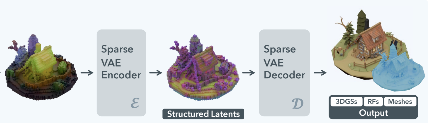
The core of this approach lies in treating the 3D shape as a tensor with a clear spatial structure. Sparse-voxel based VAE models learn local features and hierarchical structures through Convolution operations instead of a Transformer.

1. Encoder

The encoder progressively downsamples the input 3D grid ([B, C, D, H, W]) using ResBlock3d and DownsampleBlock3d (3D Convolution or 3D Pooling).

# Trellis/models/sparse_structure.py

class SparseStructureEncoder(nn.Module):
    def __init__(self, in_channels: int, latent_channels: int, channels: List[int], ...):
        super().__init__()
        # Input Layer
        self.input_layer = nn.Conv3d(in_channels, channels[0], 3, padding=1)

        # Downsampling Blocks
        self.blocks = nn.ModuleList([])
        for i, ch in enumerate(channels):
            self.blocks.extend([ResBlock3d(ch, ch) for _ in range(num_res_blocks)])
            if i < len(channels) - 1:
                self.blocks.append(DownsampleBlock3d(ch, channels[i+1]))

        # Bottleneck
        self.middle_block = nn.Sequential(...)
        self.out_layer = nn.Sequential(..., nn.Conv3d(channels[-1], latent_channels*2, 3, padding=1))

    def forward(self, x: torch.Tensor, ...):
        # x: [B, C, D, H, W], a 3D grid
        h = self.input_layer(x)
        for block in self.blocks:
            h = block(h) # Convolutions and Downsampling

        h = self.middle_block(h)
        h = self.out_layer(h)

        mean, logvar = h.chunk(2, dim=1) # Split channels in half for mean and logvar
        # ... Reparameterization Trick ...
        return z # Latent z is also a 3D grid: [B, latent_C, D', H', W']

This code is virtually identical to the Encoder structure of a typical 3D U-Net. The ResBlock3d, composed of 3D Convolutions and Skip-connections, effectively learns feature representations. The DownsampleBlock3d uses a convolution with stride=2 to halve the spatial dimensions (D, H, W) while increasing the feature dimension (C) to compress information.

What's noteworthy is the final part of the forward function. The channels of the final output h are split in half to be used as the mean and log variance (logvar) respectively. This means that the final latent representation z is also a small 'Latent Grid' of shape [B, latent_C, D', H', W']. This is a fundamental difference from the vecset-based VAE, which outputs a vector sequence. Here, the latent representation itself maintains a spatial structure.

2. Decoder: Feature Upsampling

The Decoder has a perfectly symmetrical structure to the Encoder. It takes the compressed 'Latent Grid' as input and progressively restores it to the original 3D Grid resolution using UpsampleBlock3d.

# Trellis/models/sparse_structure.py

class UpsampleBlock3d(nn.Module):
    def __init__(self, in_channels: int, out_channels: int, mode: Literal["conv", "nearest"] = "conv"):
        # ...
        if mode == "conv":
            self.conv = nn.Conv3d(in_channels, out_channels*8, 3, padding=1)

    def forward(self, x: torch.Tensor) -> torch.Tensor:
        # ...
        x = self.conv(x)
        return pixel_shuffle_3d(x, 2) # (D,H,W) -> (2D,2H,2W)

class SparseStructureDecoder(nn.Module):
    def __init__(self, out_channels: int, latent_channels: int, ...):
        super().__init__()
        self.input_layer = nn.Conv3d(latent_channels, channels[0], 3, padding=1)
        self.middle_block = nn.Sequential(...)
        self.blocks = nn.ModuleList([])
        # ... Upsampling Blocks ...

    def forward(self, x: torch.Tensor) -> torch.Tensor:
        # x: Latent Grid [B, latent_C, D', H', W']
        h = self.input_layer(x)
        h = self.middle_block(h)
        for block in self.blocks:
            h = block(h) # Convolutions and Upsampling
        h = self.out_layer(h)
        return h # Reconstructed Grid [B, C, D, H, W]

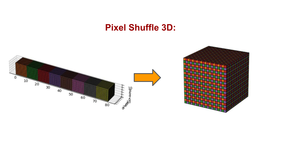
UpsampleBlock3d uses the pixel_shuffle_3d technique. This performs a role similar to 3D Transposed Convolution but is known to be more advantageous in terms of computational efficiency and avoiding checkerboard artifacts. It is a highly effective alternative for efficiently increasing spatial resolution while avoiding the potential problems of 3D Transposed Convolution.

def pixel_shuffle_3d(x: torch.Tensor, scale_factor: int) -> torch.Tensor:
    """
    3D pixel shuffle.
    """
    # 1. init state
    B, C, H, W, D = x.shape

    # 2. Channel Decomposition
    C_ = C // scale_factor**3
    x = x.reshape(B, C_, scale_factor, scale_factor, scale_factor, D, H, W)

    # 3. Dimension Re-Permutation 
    x = x.permute(0, 1, 5, 2, 6, 3, 7, 4) # (B, C_, H, scale_d, W, scale_h, D, scale_w)

    # 4. Reshaping
    x = x.reshape(B, C_, H*scale_factor, W*scale_factor, D*scale_factor)

    return x

When scale_factor=2, let's assume the initial shape of x is [B, 8C', H, W, D] (this is precisely why out_channels*8 was used in UpsampleBlock3d).

The pixel_shuffle_3d kernel performs the inverse operation of downsampling, reducing the channel dimension while doubling the spatial dimensions.

That is, through:

x = x.reshape(B, C_, scale_factor, scale_factor, scale_factor, D, H, W)
x = x.permute(0, 1, 5, 2, 6, 3, 7, 4)

the order of the tensor's dimensions is shuffled, bringing the spatial information that was in the channel dimension next to the actual spatial dimensions.

Before permute: (B, C', scale_h, scale_w, scale_d, H, W, D) (logical order)
After permute: (B, C', H, scale_h, W, scale_w, D, scale_d)

Now, immediately after each spatial dimension (H, W, D), the scale_factor that will expand that space is positioned, and the data's order in memory is rearranged. Afterward, reshaping merges adjacent dimensions, so (H, scale_h) becomes H*2, (W, scale_w) becomes W*2, and (D, scale_d) becomes D*2.

As a result, the tensor that was [B, 8C', H, W, D] is transformed into a tensor where the channel dimension is reduced to C' but the spatial resolution is increased by a factor of 2 in each dimension to [B, C', 2H, 2W, 2D].

Why is it better than Transposed Convolution?

Computational Efficiency: pixel_shuffle mainly consists of memory rearrangement operations (reshape, permute), making it very computationally inexpensive. The main computation is just a single standard Conv3d performed beforehand.
Checkerboard Artifacts: Transposed Convolution has a chronic problem of creating checkerboard-like grid noise in the output due to the way its kernel overlaps. This can significantly degrade visual quality, especially in generative models. pixel_shuffle avoids kernel overlap as each pixel is calculated independently and then rearranged, thus preventing such artifacts.
Training Stability: Simpler, more direct operations tend to facilitate a smoother gradient flow, making training more stable.

vs. VecSet-Based VAE

Do you remember the various problems associated with the VecSet-based VAE discussed earlier? The advantages of the Sparse-Voxel based VAE become clear when compared to the vecset-based approach.

No Sampling Error: Since the input itself is an SDF grid containing the overall geometric information of the original mesh, there is no information loss due to sampling. (Of course, quantization error from the initial preprocessing step exists, but this is outside the scope of the VAE model's training.)
Well-posed Problem: The model doesn't need to solve the difficult problem of "inferring the space between points." It simply needs to focus on restoring an "SDF grid to an SDF grid," i.e., a compression and reconstruction problem within the same modality.
No Modality Conversion Burden: Since the input and output formats are the same, the VAE can focus solely on the efficient compression and reconstruction of information.

In conclusion, the summary is as follows:

"While a Vecset-based VAE is a 'Modality Conversion + Compression' model that entails information loss and difficult inference problems, a Sparse Voxel VAE is a much more well-defined 'Compression' model."

Due to this fundamental difference, the Sparse Voxel VAE is structurally in a much more advantageous position in terms of shape preservation and detail reconstruction. While the advantage of the vecset-based approach lies in its input data flexibility (it can directly process point clouds, not just meshes), it is true that it has more structural limitations in generating high-quality 3D shapes. This is being demonstrated by the recent progress in sparse-voxel based research, which we will discuss in more depth in [Section E].

Summary

Sparse Voxel VAE: Maintains the 3D spatial grid structure. The latent is also a 3D grid of shape [B, C, D, H, W] -> this requires 3D Patchifying when designing a DiT.

It does not suffer from the modality conversion problem faced by Vecset-based VAEs, which allows for flexible scalability.

D. DiT on Latent Space

Now, let's examine how DiT-based generative models are designed differently on top of the two types of latent spaces created by the VAEs.

D.1. Diffusion Transformer

The innovation of DiT in 2D image generation began by adopting the methodology of the Vision Transformer (ViT). ViT divides an image into fixed-size patches, treats each patch as a single token, and uses them as the input sequence for a Transformer.

This process is clearly visible when looking at the original 2D DiT code:

# From Original DiT by Facebook Research
class DiT(nn.Module):
    def __init__(self, input_size=32, patch_size=2, ...):
        super().__init__()
        # ...
        self.x_embedder = PatchEmbed(input_size, patch_size, in_channels, hidden_size, bias=True)
        # ...

    def forward(self, x, t, y):
        # x: (N, C, H, W) tensor of spatial inputs (images)
        # The first step is to patchify the image `x`
        x = self.x_embedder(x) + self.pos_embed  # (N, T, D), T = num_patches
        # ...

The x_embedder uses nn.Conv2d to divide the image into patches and applies a linear transformation to each patch to create a token sequence of shape (N, T, D). In other words, a Patchify process that converts spatial Grid data into a token sequence is essential.

With this clearly in mind, let's look at how subsequent DiTs in 3D are designed.

D.2. VecSet DiT

Recall from the previous step that we used a vecset-based VAE to transform a 3D Mesh into a vecset-based latent, which is a latent vector in the form of a PointCloud. The shape of this data is [Batch, Num_points, Latent_dim].

This means that the output of the Vec-set VAE is already a token sequence of shape [B, N, C]. Therefore, the DiT can process this sequence directly, and the Patchify process required in the 2D image DiT becomes unnecessary.

In this case, the DiT model is simply composed of a set of standard Transformer blocks consisting of cross-attention and self-attention, with perhaps a simple linear layer to match the feature dimensions.

# DiT w/ vecset-based VAE
# ...
class DiTLayer(nn.Module):
    def __init__(self, dim, num_heads, qknorm=False, gradient_checkpointing=True, qknorm_type="LayerNorm"):
        super().__init__()
        self.dim = dim
        self.num_heads = num_heads
        self.gradient_checkpointing = gradient_checkpointing

        self.norm1 = nn.LayerNorm(dim, eps=1e-6, elementwise_affine=False)
        self.attn1 = SelfAttention(dim, num_heads, qknorm=qknorm, qknorm_type=qknorm_type)
        self.norm2 = nn.LayerNorm(dim, eps=1e-6, elementwise_affine=False)
        self.attn2 = CrossAttention(dim, num_heads, context_dim=dim, qknorm=qknorm, qknorm_type=qknorm_type)
        self.norm3 = nn.LayerNorm(dim, eps=1e-6, elementwise_affine=False)
        self.ff = FeedForward(dim)
        self.adaln_linear = nn.Linear(dim, dim * 6, bias=True)
   # ...

class DiT(nn.Module):
    def __init__(self, latent_dim=8, hidden_dim=1024, ...):
        super().__init__()
        # No PatchEmbed layer, but projection linear layer!
        self.proj_in = nn.Linear(latent_dim, hidden_dim) # Simple projection
        # timestep encoding
        self.timestep_embed = TimestepEmbedder(hidden_dim)

        # transformer layers
        self.layers = nn.ModuleList(
            [DiTLayer(hidden_dim, num_heads, qknorm, gradient_checkpointing, qknorm_type) for _ in range(num_layers)]
        )

        # project out
        self.norm_out = nn.LayerNorm(hidden_dim, eps=1e-6, elementwise_affine=False)
        self.proj_out = nn.Linear(hidden_dim, latent_dim)
    # ...

In some interpretations, the point cloud sampling itself could be considered to imply token sampling.

D.3. Sparse Voxel DiT

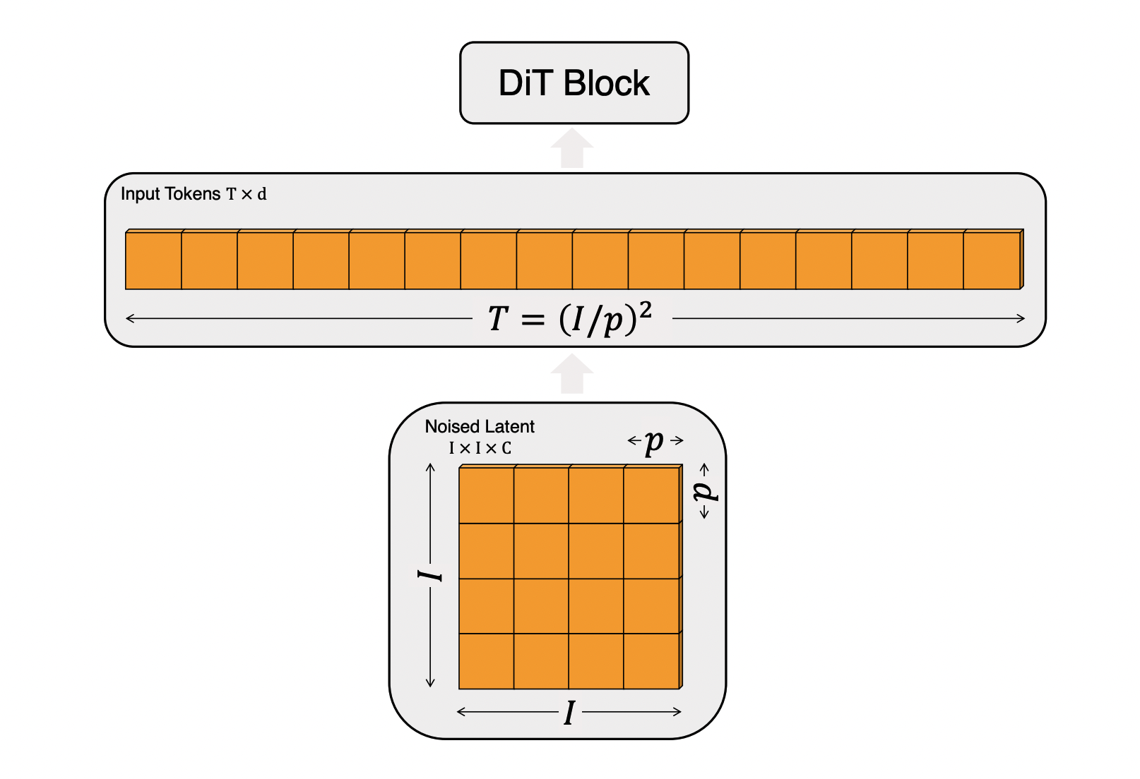
On the other hand, the output of the Sparse Voxel VAE is a 3D Latent Grid of shape [B, C, D, H, W]. For a Transformer to process this data, which has a spatial structure, a Patchify process is once again necessary, just like in the 2D DiT.

# From Trellis (Voxel-based)
class SparseStructureFlowModel(nn.Module):
    def forward(self, x: torch.Tensor, ...):
        # x: [B, C, D, H, W], a 3D grid latent space
        h = patchify(x, self.patch_size) # Patchify the 3D grid
        h = h.view(*h.shape[:2], -1).permute(0, 2, 1).contiguous()
        h = h + self.pos_emb[None] # Add 3D positional embeddings
        # ... Transformer blocks process the token sequence ...
        h = unpatchify(h, self.patch_size) # Unpatchify back to a grid
        return h

The 3D Voxel Grid x is divided into 3D patches, which are then converted into a token sequence and fed into the Transformer.

Trellis's patchfy function:

def patchify(x: torch.Tensor, patch_size: int):
    """
    Patchify a tensor.

    Args:
        x (torch.Tensor): (N, C, *spatial) tensor
        patch_size (int): Patch size
    """
    DIM = x.dim() - 2
    for d in range(2, DIM + 2):
        assert x.shape[d] % patch_size == 0, f"Dimension {d} of input tensor must be divisible by patch size, got {x.shape[d]} and {patch_size}"

    x = x.reshape(*x.shape[:2], *sum([[x.shape[d] // patch_size, patch_size] for d in range(2, DIM + 2)], []))
    x = x.permute(0, 1, *([2 * i + 3 for i in range(DIM)] + [2 * i + 2 for i in range(DIM)]))
    x = x.reshape(x.shape[0], x.shape[1] * (patch_size ** DIM), *(x.shape[-DIM:]))
    return x

The spatial information maintained at the VAE stage is converted into a sequence at the Transformer's input stage! This means that Trellis's DiT can be seen as a 3D extension of the 2D DiT.

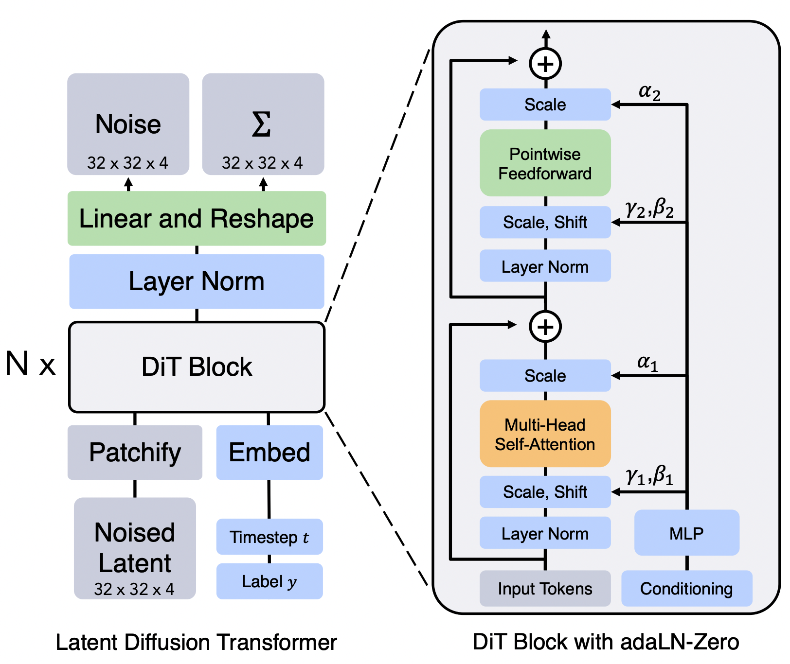
Figure from Scalable Diffusion Models with Transformers

D.4. Training with Rectified Flow

Now let's explore how this DiT is trained.

As mentioned in a previous post, the Shape generation models in the recent 3D Generative Pipeline operate on the Rectified Flow framework.

Source ($z_0 \sim p_0$): The source distribution (typically a standard normal distribution $\mathcal{N}(0, I)$).
Target ($z_1 \sim p_1$): A target sample from the target distribution (the data's latent space distribution $q_{data}$).

Here, the model's training objective is to predict the transformation path from the source distribution to the target distribution.

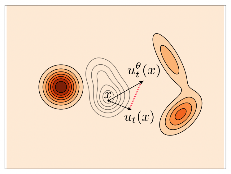
Specifically, Rectified Flow defines a path of probability distributions $p_t$ that changes over time $t$, and assumes this path to be the simplest possible form: a linear interpolation.

$$ z_t = (1-t)z_0 + t z_1 $$

Given a point $z_t$ at a specific time $t$ on this path, the role of the model (DiT) is to predict the velocity vector of this linear path. The velocity of this path can be found by differentiating with respect to time $t$,

$$ v_t = \frac{d z_t}{dt} = z_1 - z_0 $$

which shows that this velocity is always a constant vector $v = z_1 - z_0$, independent of time $t$ or position $z_t$. Therefore, the model $v_\theta(z_t, t)$ is trained to predict this constant velocity vector $z_1 - z_0$ given the current position $z_t$ and time $t$.

If we formulate the above into a general Objective Function, we can see that it becomes what is commonly known as the Conditional Flow Matching (CFM) Loss.

$$ \mathcal{L}_{CFM}(\theta) = \mathbb{E}_{t \sim U(0,1), z_0 \sim p_0, z_1 \sim p_1} \left[ || v_\theta(z_t, t) - (z_1 - z_0) ||^2 \right] $$

This is the core idea of Rectified Flow.

The training_step code of an actual 3D Flow Matching model also faithfully reflects this CFM idea.

# From Model.training_step
def training_step(self, data, iteration):
    # ...
    # 1. Get Condition `c` from image
    cond = self.get_cond(cond_images.view(-1, C, H, W), cond_num_part)

    with torch.no_grad():
        # 2. Get Target Latent `z_1` from VAE
        # posterior = self.vae.encode(data)
        latent = posterior.mode().float().nan_to_num_(0)  # z_1

        # 3. Create a point `z_t` on the straight path
        #    z_t = t*z_1 + (1-t)*z_0, where z_0 is noise
        noisy_latent, noise, timesteps = self.scheduler.add_noise(
            latent, self.config.logitnorm_mean, self.config.logitnorm_std
        ) # noisy_latent is z_t, noise is z_0

    # 4. Predict the velocity vector with DiT
    noisy_latent = noisy_latent.to(dtype=self.precision)
    model_pred = self.dit(noisy_latent, cond, timesteps)

    # 5. Calculate Loss
    # The velocity vector v = z_1 - z_0 = latent - noise
    # The code uses target = noise - latent, which is -v. This is also a valid objective.
    target = noise - latent
    loss = F.mse_loss(model_pred.float(), target.float())

    return output, loss

Condition: Extract DINOv2 features from the input image to create the image condition $c$.
Target $z_1$: Use a pre-trained VAE to encode the latent ($z_1$) from the Ground Truth 3D data.
Trajectory $z_t$: The scheduler.add_noise function randomly samples a time $t$ and uses the formula $z_t = t \cdot z_1 + (1-t) \cdot z_0$ to generate a point noisy_latent ($z_t$) between the noise $z_0$ and the target $z_1$.
Velocity Estimation: The DiT model $v_\theta$ takes $z_t$, condition $c$, and time $t$ as input to predict the velocity vector (or its negative) (model_pred).
Loss: Calculates the MSE Loss between the predicted velocity model_pred and the actual velocity target to minimize the $\mathcal{L}_{CFM}$ defined above.

Instead of the complex score-matching objective function of diffusion models, using a very simple and clear MSE Loss—"predict the direction of the straight path"—enables fast and stable training.

For a detailed physical and mathematical explanation of Rectified Flow and Flow Matching, please refer to the following: From Flow Matching to Optimal Transport: A Physics-based View of Generative Models

This explains the mathematical definitions of Flow and connects Rectified Flow's choice of a straight path to physics-based concepts (Optimal Transport, Least Action Principle).

E. Discussion: Semantic vs. Spatial

So far, we have analyzed in detail the VAE and DiT architectures for 3D generation, as well as their training methodology. Taking a step further, let's discuss a key question the research community is currently posing about the future direction of 3D generative models.

"To build a good 3D generative model, what should we align with? The Semantic Structure of a Vision Foundation Model (2D), or the inherent Spatial Structure of 3D?"

E.1. Reconstruction vs. Generation Dilemma

A recent study in the 2D image generation field, VA-VAE (Vision-Aligned VAE), presents an important observation.

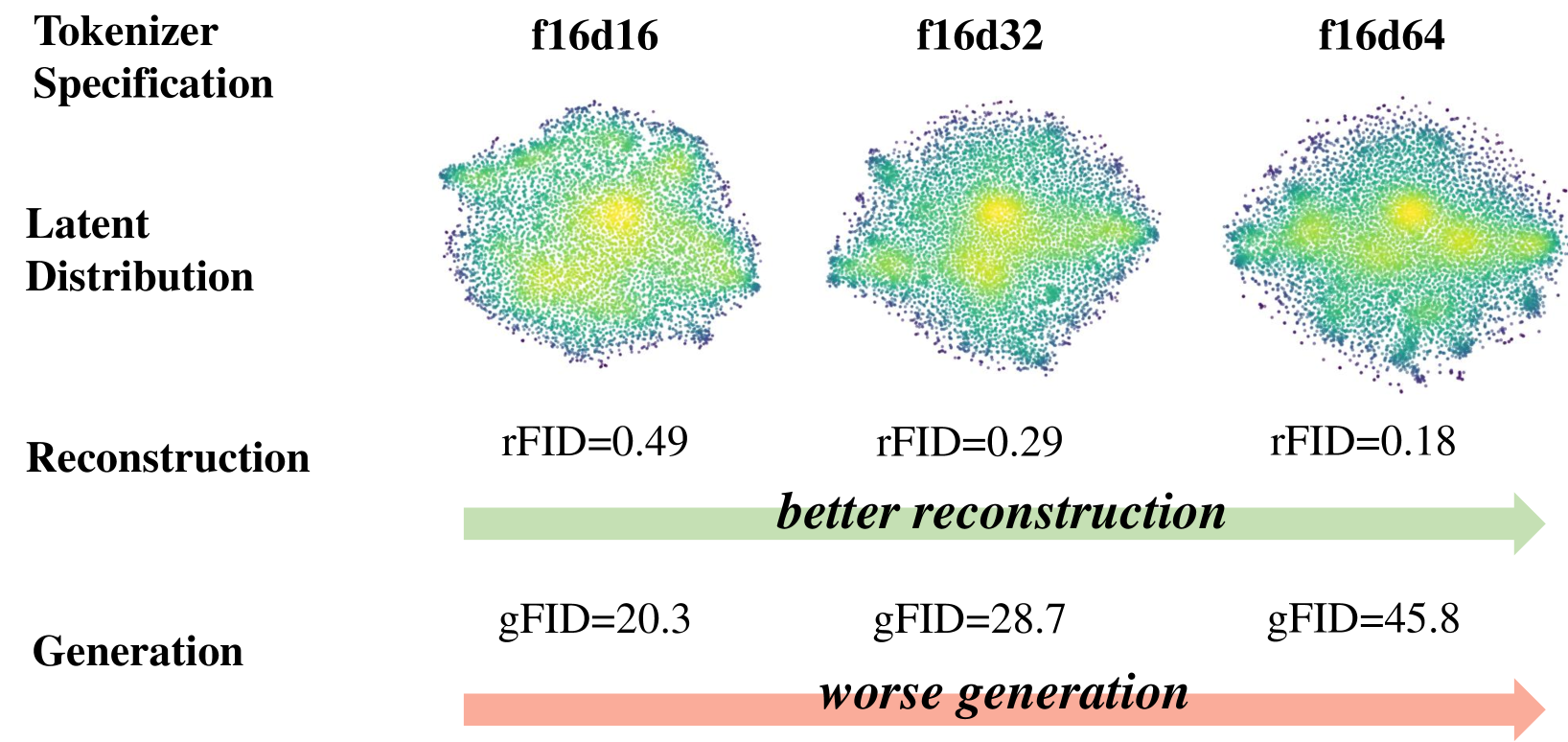
As the VAE's latent space acquires a higher dimension, the original image reconstruction quality improves, but the performance of the generative model (DiT) that has to learn on this complex latent space actually degrades.

Why does this phenomenon occur? The authors argue it's because the latent space of a VAE trained solely for high reconstruction quality is not semantically well-structured. In other words, the vectors in the latent space are scattered chaotically, making it very difficult for the generative model to learn a specific concept like 'cat'.

VA-VAE's solution is simple yet effective: align the VAE's latent space with the feature space of a Vision Foundation Model (e.g., DINO). Simply adding a loss that increases the cosine similarity between the latent vector and the DINO feature vector during VAE training provides the following benefits to the latent space:

Semantically Rich & Well-structured: Semantically similar objects cluster together in the latent space.
Faster Convergence: Thanks to the semantically structured latent space, the DiT can focus on learning relationships between high-level semantic units instead of low-level pixel combinations, leading to dramatically faster training. (VA-VAE: 1400 epochs → 80 epochs)

E.2. VA-VAE and 3D Generation

The Vecset-based VAE, which uses Point Clouds and focuses solely on reconstructing 3D shapes, has aspects similar to the 'reconstruction-specialized' VAE pointed out by VA-VAE. This leads to the hypothesis that since the DiT (Flow Model) must inefficiently search a vast, unstructured latent space to generate a shape matching the input condition (2D), its convergence may be slow and its performance limited.

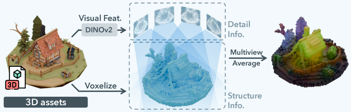
On the other hand, Trellis can be seen as having already implemented an idea similar to VA-VAE in 3D with its concept of SLAT (Structured Latent). SLAT uses the DINO feature map itself as the VAE's training target, creating a semantic latent space that possesses spatial structure. In essence, the approach is: "DINO is already good enough, so let's just map it directly onto the 3D space!"

However, this method has the problem of effectively splitting the VAE's latent space in two. That is, it is composed of Structure, which determines 'where the shape exists?', and Feature, which determines 'what exists there?'. This leads to a complex 2-stage generation pipeline.

1) Structure Generation: First, a model must generate the indices of the Sparse Structure, which determines which voxels are activated. Trellis trains a separate Conditional Flow Matching (CFM) model for this purpose.
2) Feature Generation: Conditioned on the Sparse Structure generated in the first stage, a second model (a DiT-like Transformer) generates the SLAT, i.e., the projected DINO feature, corresponding to each activated voxel location. The training objective of this model is the highly complex mapping from 'Gaussian Noise → the projected DINO feature of the corresponding voxel'.

As a result, the VAE was now tasked with the much more difficult challenge of reconstructing not just a simple 3D structure (SDF values), but the complex projected DINO features themselves for each voxel. This increased the model's capacity and training burden. The fact that Trellis was limited to a relatively low resolution of $64^3$ was not so much a technical choice as an inevitable consequence of the task of reconstructing DINO features. Consequently, the detail in the generated 3D shapes was bound to be blurry and smoothed out.

This has been demonstrated by the overwhelming 3D shape generation capabilities of models like Hunyuan 3D 2.0 and TripoSG released earlier this year, which surpassed Trellis.

E.3. Back to Spatial Fundamentals?

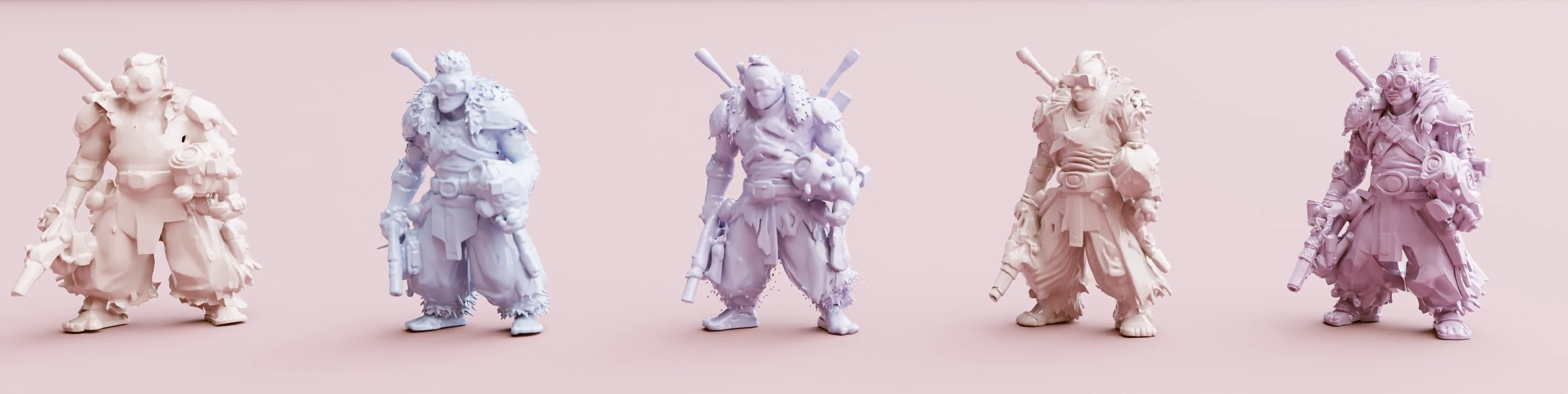
However, recent follow-up studies to Trellis (such as SparseFlex, Direct3D-S2, and Sparc3D) are showing a noteworthy change.

Trellis / Hunyuan-2.0 / TripoSG / Hi3DGen / Direct 3D-s2

These models boldly discard Trellis's SLAT, i.e., the direct alignment with DINO, and instead focus their technical efforts on increasing the resolution of the 3D latent grid (e.g., to 256^3) and more efficiently compressing 3D spatial relations.

This may be evidence that for 3D shape generation, capturing the part-whole relationships and topological structure of the 3D space itself at high resolution is more important than semantic alignment with a 2D Vision Foundation Model. The 'semantic' information of a 2D image and the 'structure' of a 3D shape are fundamentally different kinds of information, and the core of 3D shape generation lies in the latter.

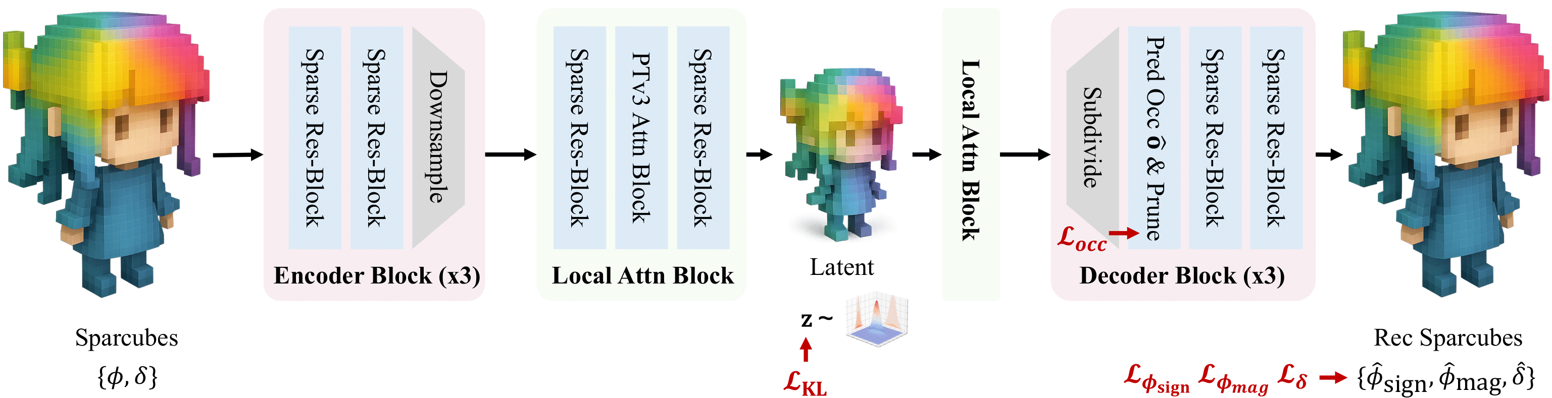
Figure: Sparc3D's efficient Sparconv-VAE, which directly compresses Voxel indices and SDF values instead of DINO features.

These two contrasting viewpoints can be thought of as diverging into two potential paths for the future of 3D generative models:

By applying the ideas of VA-VAE to vecset-based models, can we create a semantically structured latent space to achieve both faster training and better performance?
Or, as is the current trend, is the answer to part ways with Vision Models and focus purely on modeling the spatial and topological properties of 3D data at high resolution?

I believe the process of finding the answer to this question will be the central focus of the next generation of 3D Foundation model research.

Conclusion

In this article, we have conducted a deep comparative analysis of the internals of DiT-based models for 3D shape generation, focusing on the differences in data representation (Vecset vs. Voxel).

The next article in this series was planned to cover practical strategies for efficiently training massive 3D Generative Models by setting up a Multi-Node, Multi-GPU environment and using memory optimization libraries like DeepSpeed and FSDP with their sharding strategies.

While I originally planned to cover multi-node training as a follow-up to this article, I felt a deep need to explain the importance of Flow Matching more thoroughly (it was briefly in the middle of Section D, but a detailed explanation of Flow became too long and threatened to take over the entire article...). Therefore, I have spun it off into a separate article that explains Flow A-to-Z in detail. In the next article, I provide a detailed explanation from the definition of Normalizing Flow to Rectified Flow, and connect it to Optimal Transport to explain in detail why Rectified Flow adopted a straight-line path.

Stay Tuned!

References

Vecset-based VAE

3D Generation w/ vecset-based VAE

Sparse-Voxel VAE (& its 3D Generation)