---

Introduction: Rise of 3D Generative AI

Since the latter half of 2024, starting with CLAY (Rodin), a wave of 3D Generative Models has been released, including Hunyuan3D, Trellis, TripoSG, Hi3DGen, and Direct3D-S2.

All of these methods follow a common design blueprint:

• Shape Generation: A generative model (Diffusion, Flow) for the '3D Shape (Mesh)'.

• Texture Generation: Shape-conditioned, multi-view consistent image generation (though some models employ slightly different designs for PBR textures, the fundamental framework is similar).

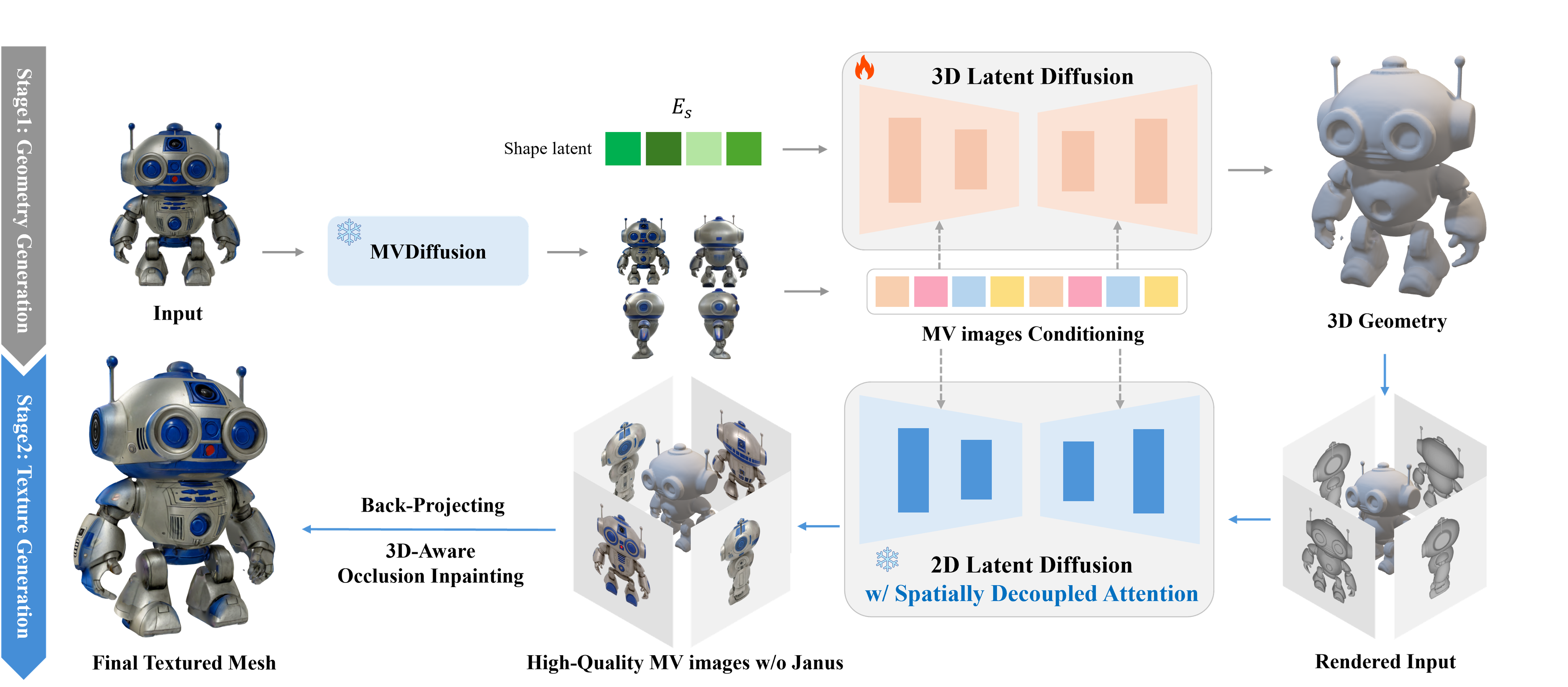
This can be interpreted as decoupling the 3D asset creation process into 1) Shape Generation ↔︎ 2) Texturing, which allows for the application of the proven '2D Generative Model' methodology (Latent Generative Models).

In other words, similar to 2D generative models, a 3D shape is created using a high-quality latent space (via a VAE to compress computational cost) and a generative model trained on this latent space (Diffusion or Rectified Flow). A texture is then generated using a multi-view consistent image generation model conditioned on the created shape. This approach has delivered tremendous fidelity improvements and has become the industry standard, replacing previous lifting-based methods and NeRF/GS-based reconstruction models (LRM, LGM). (cf: Is the Era of NeRF and SDS in 3D Generation Coming to an End?, The Age of 3D Generative Models)

To build such a 3D Generative Foundation Model, one needs not only a fundamental understanding of generative modeling theory and coding skills but also a deep comprehension of the unique properties of 3D data and the ability to handle complex pre/post-processing workflows.

The complexity of 3D data can be a significant moat for newcomers to the domain. Therefore, this article series aims to minimize that difficulty by providing a detailed, from-scratch guide on how to build a 3D generation scheme.

As the first post in the series, today's article will focus on the pre-processing of 3D data.

---

A. Dataset

A fundamental point to grasp is that 3D data is significantly more scarce than 2D images. The release of the Objaverse dataset, which aggregates license-free assets from platforms like GitHub and Sketchfab, has been a game-changer. Most of the aforementioned methods use this dataset as their primary source for 3D generation.

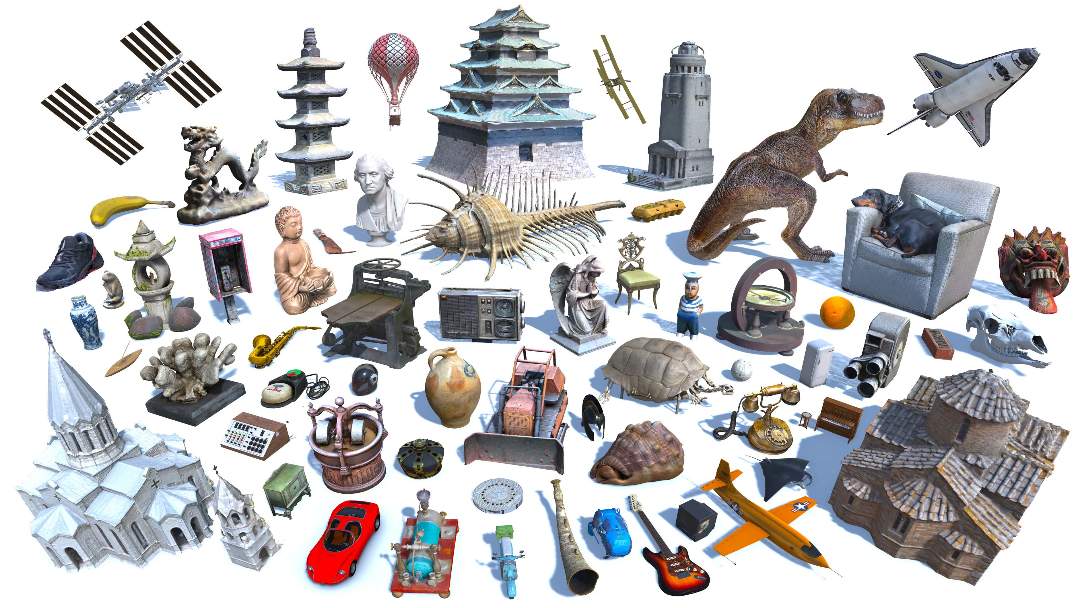
Although Objaverse contains over 10M+ 3D assets (polygonal meshes), a large portion consists of low-quality assets that are not conducive to training. Consequently, rather than using the entire dataset, researchers filter for high-quality assets based on their own criteria.

Since 3D data instances can be quite large, I recommend using publicly available filtered subsets instead of implementing a personalized filtering pipeline.

Two convenient Objaverse subsets are:

• Trellis-500K

• Step1X-800K

These subsets contain the Objaverse UIDs that Trellis and Step1X, respectively, used to train their 3D generative models.

pip install objaverse pandas

You can download the data as follows (warning: the dataset is extremely large, around ~10TB).

import os
import pandas as pd
import objaverse.xl as oxl

def download(metadata, output_dir='/temp'):    
    os.makedirs(os.path.join(output_dir, 'raw'), exist_ok=True)

    # download annotations
    annotations = oxl.get_annotations()
    annotations = annotations[annotations['sha256'].isin(metadata['sha256'].values)]
    
    # download and render objects
    file_paths = oxl.download_objects(
        annotations,
        download_dir=os.path.join(output_dir, "raw"),
        save_repo_format="zip",
    )
    
    downloaded = {}
    metadata = metadata.set_index("file_identifier")
    for k, v in file_paths.items():
        sha256 = metadata.loc[k, "sha256"]
        downloaded[sha256] = os.path.relpath(v, output_dir)

    return pd.DataFrame(downloaded.items(), columns=['sha256', 'local_path'])

metadata = pd.read_csv("hf://datasets/JeffreyXiang/TRELLIS-500K/ObjaverseXL_github.csv")
download(metadata)

On a side note, TripoSG built its own high-quality dataset of 2M assets using the following data curation rules:

• Scoring

  • Randomly select 10K 3D models and render 4-view normal maps (using Blender).
  • Hire 10 professional 3D modelers to manually score the models from 1 to 5.
  • Use this labeled data to train a linear regression scoring model (with CLIP and DINOv2 features as input).

• Filtering

  • Remove meshes where different surface patches are classified as a single plane (likely calculated using normal vectors and checking if patch centers lie on the plane).
  • For animated models, fix the model to frame 0 and remove it if significant rendering errors occur.
  • For scenes with multiple objects, use connected component analysis to isolate and remove extraneous objects (likely using functionality from trimesh).

Furthermore, they employed advanced pre-processing techniques like training an orientation model to ensure all meshes face forward and using their proprietary texturing model to generate pseudo-textures for untextured models, which were then used as diffuse maps.

From hiring a team of 10 3D modelers for labeling to training specialized scoring and orientation models, this level of curation is nearly impossible for an individual to replicate...

---

B. Pre-processing for the Shape VAE

B.1. 3D Representation

Once the data is prepared, the most critical prerequisite for training a 3D Generative Model is to convert every 3D mesh into a Normalized, Watertight Mesh. To understand why all meshes must be made watertight, let's first examine the characteristics of 3D representations.

3D representations can be broadly divided into two categories, each with distinct properties:

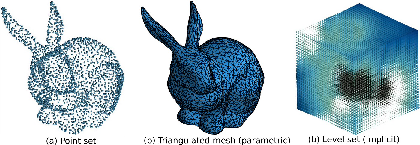
• Implicit: SDF (Signed Distance Field), UDF, NeRF, …

  • Continuous
  • Easy to decide inside ↔︎ outside
  • Hard to sample (render) → ultimately requires conversion to an explicit form

• Explicit: Polygonal mesh, occupancy grid (voxel), Gaussian Splatting, …

  • Discrete
  • Hard to decide inside ↔︎ outside
  • Easy to sample (render)

Among these, the mesh is an explicit representation, specifically defined by a set of:

• $V$: vertices (3D vectors)
• $E$: edges (pairs of vertex indices)
• $F$: faces (N-tuples of vertex indices)

---

B.2. VAE for 3D: The Vecset-based VAE

Let's revisit the primary objective of training a 3D Generative Model for shapes.

Before we can train a Diffusion or Flow model, we need a well-defined latent space. As in 2D, the need for such a space arises from two factors: 1) reducing computational cost and 2) the fact that neural networks train more effectively on a semantically meaningful, continuous space.

From this perspective, a 3D Mesh is not an ideal domain for a VAE to learn a latent space. VAEs, being neural networks, are optimized for fixed-size vectors or tensors. But what about meshes? The number of vertices ($V$), edges ($E$), and faces ($F$) varies from model to model, making it extremely difficult to define a stable input/output structure for a VAE.

Furthermore, we must consider the inherent shift/rotation-invariance of a mesh. If you translate or rotate the vertices of a mesh, it is still the same object. This means the mesh's vertices are translation/rotation invariant, and using them directly as a learning objective would likely lead to highly unstable training.

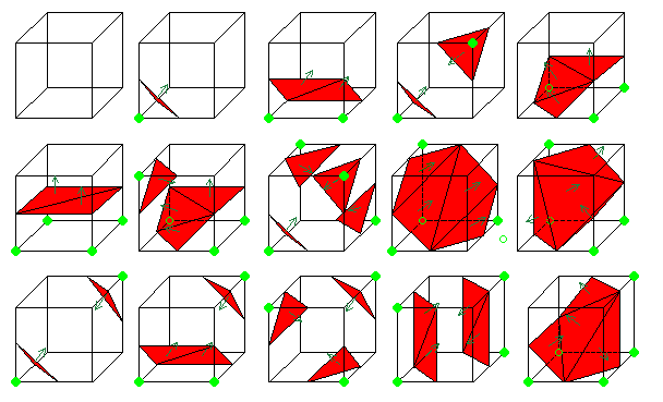
Therefore, vecset-based VAEs in 3D Generative Models adopt the following design (figure from 3DShape2vecset):

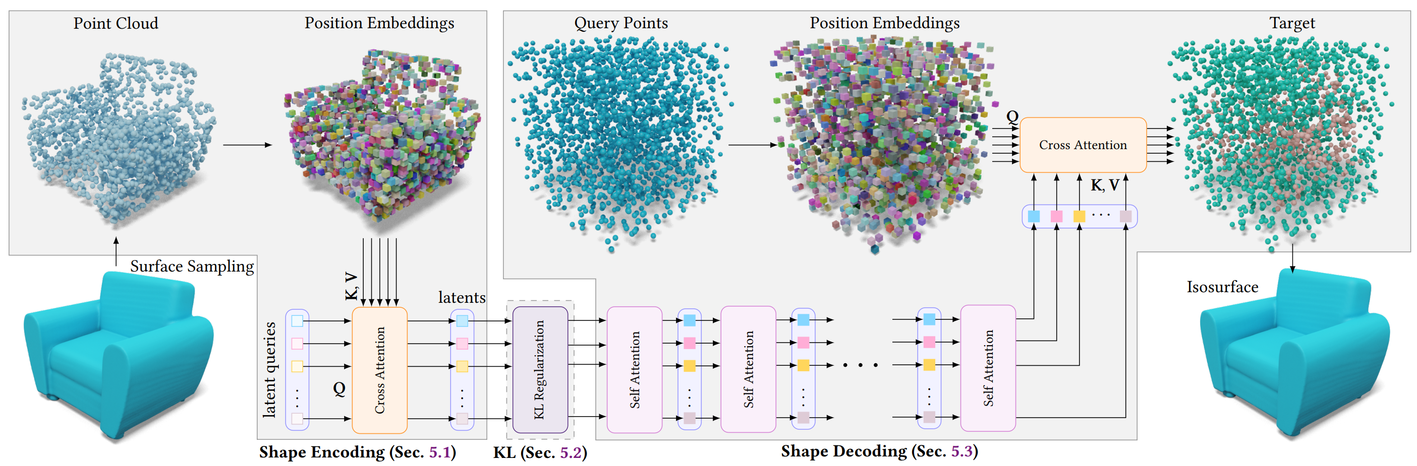
• Input: A point cloud sampled from the mesh's surface.

• Processing: Applying Fourier features (positional encoding) to the points allows the neural network to focus solely on the relative relations between points, ensuring stationary training. This removes the ambiguity caused by the mesh's translation/rotation invariance. (cf: Fourier Features Let Networks Learn High-Frequency Functions in Low-Dimensional Domains)

• Training: The VAE learns a latent space through the encode ↔︎ decode reconstruction process on these point cloud samples. (The bottleneck space, learned with a KL divergence loss, becomes the learnable space for the subsequent Diffusion/Flow model).

In this process, the VAE decoder outputs not a mesh representation, but an Implicit Representation, specifically an SDF or an Occupancy Field.

Since an implicit representation defines space as a function, the VAE decoder is trained as a parametric model that approximates the SDF from a latent vector. This makes it easy to query the SDF on a voxel grid and reconstruct a mesh using algorithms like Marching Cubes.

But what is the essential characteristic of an Implicit Representation? It is that it's:

"Easy to decide inside ↔︎ outside"

An SDF, $f(x)$, is defined as:

$$ f(x) = \begin{cases} d(x, \partial \Omega) & \text{if } x \in \Omega \\ -d(x, \partial \Omega) & \text{if } x \in \Omega^c \end{cases} \\ \\ {} \\ \text{where } d(x, \partial \Omega) = \inf_{y \in \partial \Omega} \|x - y\| $$

The SDF $f(x)$ has negative values inside the surface and positive values outside, while an Occupancy field is 1 inside and 0 outside. In short, these functions presuppose a clear distinction between 'inside' and 'outside'.

---

B.3. Watertight Meshes in Mathematics

What if the training data, the meshes, have holes or torn faces? It becomes impossible to clearly define 'inside' and 'outside'. This means we cannot determine the sign of the SDF or the 0/1 value of the Occupancy field. A model cannot learn effectively from such ambiguous ground truth.

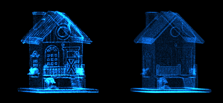
• Fig. Non-Watertight / Watertight

This is why we must ensure every mesh is 'watertight'. Mathematically, this is defined as:

"Every edge is shared by exactly two faces."

This is the minimum condition for a mesh to be a topologically stable 2-Manifold. A 2-Manifold is a space where any point on the surface, when zoomed in sufficiently, looks like a flat 2D disk. (This is the same reason flat-earthers think the Earth is flat—it's a 2-Manifold!).

This concept is further clarified by the cornerstone of topology, the Euler Characteristic.

For any closed manifold, i.e., a Watertight Mesh, the relationship between the number of vertices ($V$), edges ($E$), and faces ($F$) is always:

$$ V - E + F = 2 - 2g $$

(Here, $g$ is the number of Genus (handles or holes)).

• $g=0$ (e.g., Sphere): $V - E + F = 2$

• $g=1$ (e.g. Torus): $V - E + F = 0$

For a convex manifold with $g=0$, the formula $V - E + F = 2$ is well-known (e.g., a cube: $V=8, E=12, F=6$). We can easily generalize this by considering the process of adding a hole, which explains the $-2g$ term.

1. Consider a watertight mesh with $g=0$ (Euler characteristic = 2).
2. Remove two faces from its surface ($\triangle F = -2$). The mesh becomes non-watertight, and the value of $V-E+F$ decreases by 2.
3. Now, connect the boundaries of the two holes with a tube to make it watertight again. Since the number of new faces ($n$) equals the number of new edges ($n$), the value of $V-E+F$ remains unchanged ($\triangle V-\triangle E+ \triangle F = 0-n+n = 0$).

The crucial point is that this formula only holds for watertight meshes. A non-watertight mesh has a boundary, so the formula does not apply.

Therefore, having a mix of watertight and non-watertight objects in the VAE's training dataset means we are forcing the model to learn from topologically distinct categories of objects, even if they look similar to us. This prevents the VAE from forming a consistent latent space and destabilizes training.

Consequently, ensuring the watertightness of all meshes is the most fundamental pre-processing step for stable 3D generative model training.

The 'voxelization' step in methods like Trellis and Direct3D-S2, which use a spatial voxel grid, serves a similar purpose. The process of determining activated voxels reduces the topological ambiguity of the 3D representation. A detailed comparison between vecset-based VAEs and spatial voxel-based VAEs will be covered in a future post in this series.

---

B.4. How to Make it Watertight

So, we now understand the mathematical and topological reasons 'why' we need watertight meshes. The question that remains is:

'How do we make a non-watertight mesh watertight?'

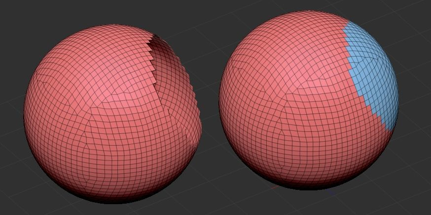
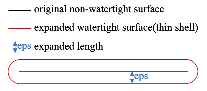
A well-known implementation, as seen in Dora, uses an algorithm that effectively wraps the entire original mesh in a thin, closed shell. (cf: Dora's to watertightmesh.py)

diffdmc = DiffDMC(dtype=torch.float32).cuda()
vertices, faces = diffdmc(grid_udf, isovalue=eps, normalize= False)

While it's difficult to determine if a point is inside or outside a non-watertight mesh, calculating the unsigned distance field (UDF) to its surface is straightforward. This method first computes the UDF, then creates a thin shell offset from the original surface by a small eps. It then treats everything within this shell (UDF < eps) as 'inside', effectively creating a pseudo-isosurface. This is what the isovalue=eps parameter in Differentiable Dual Marching Cubes does. However, this introduces not only quantization errors but also results in a mesh that is dilated and distorted by eps from the original surface.

Another, more robust method involves calculating the UDF and then using the flood-fill algorithm to convert it into a watertight mesh. While conceptually similar to reconstructing a mesh with a non-zero isovalue, this approach provides a clearer algorithmic intuition. Let's describe this method.

Core Idea: Mesh Reconstruction

Fundamentally, this algorithm is based on the idea of wrapping the original mesh in a thin shell. In other words, it doesn't "repair" the incomplete original mesh. Instead, it reconstructs a new, watertight mesh that mimics the original's form.

Step 1: Voxelization & Unsigned Distance Field

The first step is to convert the continuous 3D space and the variable mesh structure into a fixed-size grid that is easy to work with.

resolution = 512
grid_points = torch.stack(
    torch.meshgrid(
        torch.linspace(-1, 1, resolution, device=device),
        torch.linspace(-1, 1, resolution, device=device),
        torch.linspace(-1, 1, resolution, device=device),
        indexing="ij",
    ), dim=-1,
) # [N, N, N, 3]

Next, a Bounding Volume Hierarchy (BVH) is used to efficiently compute the unsigned distance field from every point in this grid to the mesh.

Install cubvh for efficient BVH computation:

pip install git+https://github.com/ashawkey/cubvh

Python:

vertices = torch.from_numpy(mesh.vertices).float().to(device)
triangles = torch.from_numpy(mesh.faces).long().to(device)

# 2. Build BVH for fast distance query
# using cubvh package!
BVH = cubvh.cuBVH(vertices, triangles)

# 3. Create a voxel grid and query unsigned distance
udf, _, _ = BVH.unsigned_distance(points.view(-1, 3), ...)
udf = udf.view(opt.res, opt.res, opt.res)

Let's look at a part of the unsigned_distance_kernel function inside cubvh:

__global__ void unsigned_distance_kernel(
    uint32_t n_elements, const Vector3f* __restrict__ positions,
    float* __restrict__ distances, int64_t* __restrict__ face_id, Vector3f* __restrict__ uvw,
    const TriangleBvhNode* __restrict__ bvhnodes, const Triangle* __restrict__ triangles, bool use_existing_distances_as_upper_bounds
) {
    uint32_t i = blockIdx.x * blockDim.x + threadIdx.x;
    if (i >= n_elements) return;

    float max_distance = use_existing_distances_as_upper_bounds ? distances[i] : MAX_DIST;
    Vector3f point = positions[i];

    // udf result
    auto res = TriangleBvh4::closest_triangle(point, bvhnodes, triangles, max_distance*max_distance);
    distances[i] = res.second;
    face_id[i] = triangles[res.first].id;
}

// C++/CUDA: Inside closest_triangle function
while (!query_stack.empty()) {
    // ...
    // Pruning: if a bounding box is farther than the closest triangle found so far...
    if (children[i].dist <= shortest_distance_sq) {
        query_stack.push(children[i].idx); // ...explore it.
    }
}

• BVH: A brute-force calculation of the distance between every voxel and every face is computationally expensive. cubvh first constructs a BVH tree structure, which dramatically improves search performance by pruning entire groups of distant faces from the search space (children[i].dist <= shortest_distance_sq).

• UDF: The CUDA kernel is invoked and executed in parallel across the GPU's numerous threads. Each thread takes one voxel point and calculates the unsigned distance to the nearest triangle using the BVH.

At the end of this stage, we have a 3D volume data—the UDF—that captures the shape of the original mesh. However, we still don't know which parts are 'inside' and which are 'outside'.

Step 2: Flood Fill

The Flood Fill algorithm is used to clearly delineate the interior and exterior.

Python Code:

# 1. Define the mesh "shell" or "wall"
eps = 2 / opt.res 
occ = udf < eps # Occupancy grid: True if a voxel is on the surface, i.e., make thin shell

# 2. Perform flood fill from an outer corner
#    (internally calls initLabels, hook, compress kernels)
floodfill_mask = cubvh.floodfill(occ)

# 3. Identify all voxels connected to the outside
empty_label = floodfill_mask[0, 0, 0].item()
empty_mask = (floodfill_mask == empty_label)

• Thin Shell (occ = udf < eps): Voxels very close to the original mesh surface are set to True (the wall), and the rest are set to False (empty space), creating a "shell" of the mesh. This shell may still contain the holes and gaps from the original mesh (if the gaps are larger than eps).

cubvh's floodfill kernel:

// C++/CUDA: Inside hook kernel
int best = labels[idx];
// ... check 6 neighbors ...
// idx +- 1, idx +- W, idx +- W*H
if (x > 0 && grid[idx-1]==0) best = min(best, labels[idx-1]);
// ... (5 more neighbors)

if (best < labels[idx]) {
    labels[idx] = best;
    atomicOr(changed, 1); // Mark that a change occurred
}

(Labeling & Spreading)

• Every voxel in the grid is assigned a unique ID.
• hook & compress: "Water" starts filling from a corner of the grid, [0,0,0], which is guaranteed to be outside. Each "empty space" voxel checks the labels of its 6 neighbors and updates its own label to the minimum value. This process cannot pass through the "wall" (occ=True), and its propagation speed is accelerated by the compress kernel (pointer jumping).
• Final Determination: Once propagation is complete, all voxels with the same label as [0,0,0] are confirmed to be 'exterior space' (empty_mask).

This is analogous to running a 'simulation of pouring water' from the outside of the canonical space where the mesh is defined. The holes and gaps in the non-watertight mesh are naturally "sealed" by the occ shell, and the flood fill yields a volume where the inside and outside are perfectly separated.

Step 3: Signed Distance Field

Now, we convert the UDF into an SDF that can be used by Marching Cubes.

Python Code:

# 1. Invert the empty mask to get inside + shell
occ_mask = ~empty_mask

# 2. Initialize SDF: surface is 0, outside is positive
sdf = udf - eps

# 3. Assign negative sign to the inside
inner_mask = occ_mask & (sdf > 0)
sdf[inner_mask] *= -1

• occ_mask includes both the 'wall' (shell) and the 'true interior' that was not identified as 'exterior' by the flood fill.
• sdf = udf - eps adjusts the values near the surface to be close to 0.
• Using occ_mask, the SDF values of voxels corresponding to the interior are multiplied by -1 to make them negative.

The result is a perfect Signed Distance Field where the interior is negative, the exterior is positive, and the surface is 0.

Step 4: Marching Cubes

Finally, we extract a new, watertight mesh from this perfect SDF volume.

Python Code:

# 1. Extract the iso-surface where sdf = 0
vertices, triangles = mcubes.marching_cubes(sdf, 0)

# 2. Normalize vertices and convert to a trimesh object
vertices = vertices / (opt.res - 1.0) * 2 - 1
watertight_mesh = trimesh.Trimesh(vertices, triangles)

# 3. Restore original scale and save
watertight_mesh.vertices = watertight_mesh.vertices * original_radius + original_center
watertight_mesh.export(f'{opt.workspace}/{name}.obj')

The Marching Cubes algorithm takes 3D grid data (the SDF) as input and generates a triangle mesh by finding the points where the SDF value is 0 (the isosurface). By its very definition, the output of this algorithm is always a closed surface—i.e., watertight.

---

B.5. Pointcloud Sampling

With watertight conversion complete, the final part of the mesh pre-processing stage is point cloud sampling. While uniform sampling from the mesh surface is not difficult, recent works like Dora, Hunyuan3D, and TripoSG have reported that sampling more points from salient edges significantly improves VAE reconstruction performance.

An implementation for Salient Edge Sampling (SES) is provided in the Dora github, but it requires a Blender installation and the bpy library, making the sampling process heavyweight.

Therefore, below, we will implement salient edge sampling in pure Python without relying on Blender's functionality.

Step 1: Identifying Salient Edges

• Assumption: A "salient edge" is an edge where the dihedral angle between its two adjacent faces is large.

This means we can identify 'salient edges' by calculating the dot product of the normal vectors of adjacent faces in the mesh and checking if the angle exceeds a certain threshold.

salient_edges = []
total_edge_length = 0.0

# mesh.face_adjacency stores pairs of adjacent face indices
for i, face_pair in enumerate(mesh.face_adjacency):
    face1_idx, face2_idx = face_pair
    normal1 = mesh.face_normals[face1_idx]
    normal2 = mesh.face_normals[face2_idx]
    
    angle = np.arccos(np.clip(np.dot(normal1, normal2), -1.0, 1.0))

    if angle > thresh_angle_rad:
        # mesh.face_adjacency_edges stores the vertex indices of the shared edge
        edge_vertices_indices = mesh.face_adjacency_edges[i]
        v1_idx, v2_idx = edge_vertices_indices
        
        v1 = mesh.vertices[v1_idx]
        v2 = mesh.vertices[v2_idx]
        length = np.linalg.norm(v1 - v2)
        
        if length > 1e-8:
            total_edge_length += length
            salient_edges.append((v1_idx, v2_idx, length))

As shown above, we calculate the angle between the two normal vectors by taking the arccos of their dot product.

Step 2: Initial Sampling

The first step of sampling is to sample the endpoints (vertices) of the salient edges. We iterate through the salient_edges list found in Step 1 and use the start (v1_idx) and end (v2_idx) vertex indices as our initial samples.

initial_samples = []
added_vertex_indices = set()
for v1_idx, v2_idx, _ in salient_edges:
    if v1_idx not in added_vertex_indices:
        initial_samples.append(mesh.vertices[v1_idx])
        added_vertex_indices.add(v1_idx)
    if v2_idx not in added_vertex_indices:
        initial_samples.append(mesh.vertices[v2_idx])
        added_vertex_indices.add(v2_idx)

samples = np.array(initial_samples)

Step 3: Interpolation

Since the number of vertices collected in Step 2 may be less than our target sample count, we additionally sample points along the salient edges. We assume that longer edges contain more features, so we allocate the number of extra samples to be added proportionally to the length of each edge.

num_extra = num_samples - len(samples)
extra_samples = []
if total_edge_length > 0:
    for v1_idx, v2_idx, length in salient_edges:
        # based on the edge length, proportionally distribute extra samples
        extra_this_edge = math.ceil(num_extra * length / total_edge_length)
        
        v1 = mesh.vertices[v1_idx]
        v2 = mesh.vertices[v2_idx]
        
        for j in range(extra_this_edge):
            t = (j + 1.0) / (extra_this_edge + 1.0) # Uniformly space points
            new_point = v1 + (v2 - v1) * t
            extra_samples.append(new_point)

Here, we use linear interpolation to ensure uniform sampling within each edge.

Final Step

Finally, we use FPS (Farthest Point Sampling) to select exactly num_samples points.

Install the Farthest Point Sampling package:

pip install fpsample

Python:

if len(all_samples) > num_samples:
    indices = fpsample.bucket_fps_kdline_sampling(all_samples, num_samples, h=5)
    return all_samples[indices]

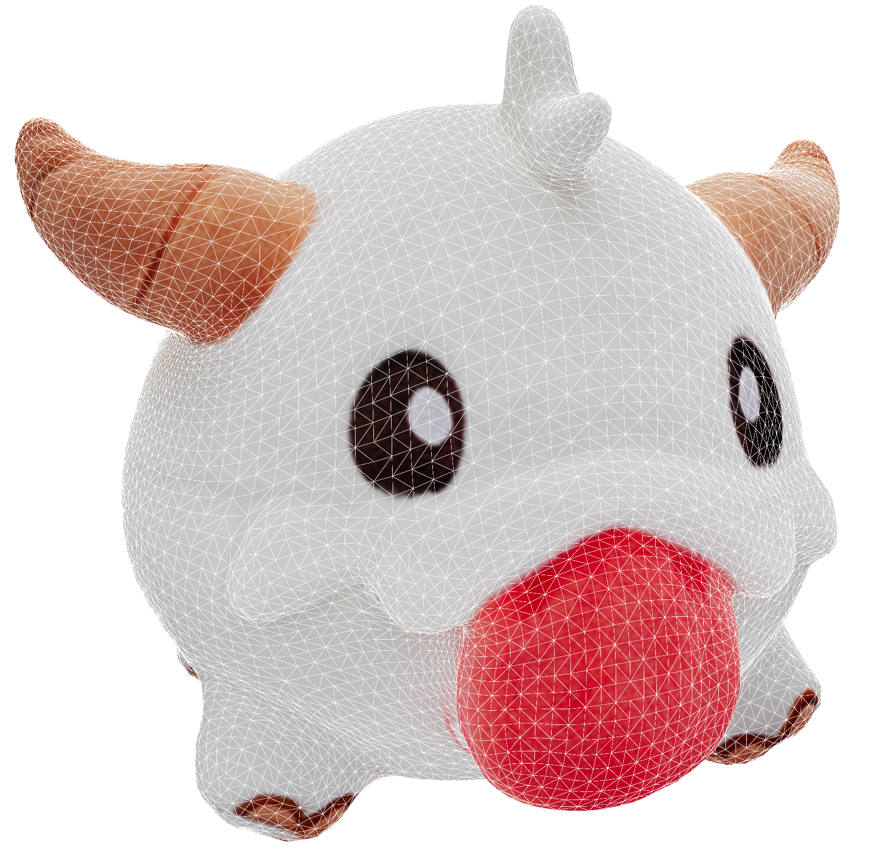
• Result (Left: Input Mesh, Right: Output Salient Sampling Point Cloud)

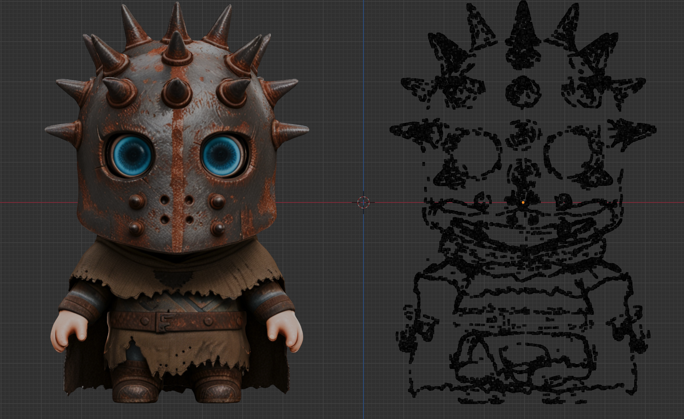
While this is a functional conceptual implementation, the meshiki package provides a much faster implementation in C++. Using it, you can perform SES directly as follows:

# pip install meshiki
from meshiki import Mesh, fps, load_mesh, triangulate

vertices, faces = load_mesh(mesh_path, clean=True)
faces = triangulate(faces)
mesh = Mesh(vertices, faces)

# sample 64K salient points
salient_points = mesh.salient_point_sample(64000, thresh_bihedral=30)

---

Conclusion

In this article, we took a deep dive into the first step of building a 3D Generative Model: data pre-processing.

In addition to the processing steps discussed above, a complete pre-processing pipeline for a 3D Generative Model also requires multi-view rendering of the mesh. This means one must also be proficient with Blender rendering scripts using tools like bpy. (cf: Blenderproc, Trellis dataset toolkits)

While not on the scale of LLMs, training a 3D Generative Model is still a cost-consuming task, typically requiring a 1B to 3B parameter model, at least 64 GPUs with 80GB+ VRAM each, and over 20TB of NAS for handling the 3D data.

However, excellent open-source models are continuously being released. To leverage these foundation models for tasks like fine-tuning or LoRA-Adapter Training while minimizing the use of the most expensive resource—GPUs—a solid command of 3D data pre-processing is absolutely essential.

Since working on the CaPa Project last year, I have been training our own 3D generative model and developing a 3D generation service based on it. We plan to announce it publicly soon, and I hope to be able to introduce it then.

The next article in this series will delve into the architectures of ShapeVAE and Flow Models, as well as strategies for efficiently training 3D Generative Models by setting up a multi-node environment and using the sharding strategies of DeepSpeed v3 and FSDP.

Stay Tuned!

---

You may also like:

• Is the Era of NeRF and SDS in 3D Generation Coming to an End? (kor)
• The Age of 3D Generative Models