---

Introduction: Rise of 3D Generative AI

2024년 하반기 이후, CLAY (Rodin) 를 기점으로 Hunyuan3D, Trellis, TripoSG, Hi3DGen, Direct3D-S2 등 수많은 3D Generative Models 들이 쏟아지고 있다.

이 모든 method 들은 다음의 설계,

• Shape Generation: '3D Shape (Mesh)' 에 대한 Generative Model (Diffusion, Flow)

• Texure Generation: Shape-conditioned Multi-view consistent Image generation (PBR texture 를 위해 조금 다른 설계를 구가하는 경우도 있지만, 일단 기본적인 골자는 비슷하다)

를 따르는데, 이는 3D asset 의 1) Shape Generation ↔︎ 2) Texturing 을 분리하여 이미 성공 공식이 있는 ‘2D Generative Model’ 의 방법론 (Latent Generative Model) 을 적용시켰다고 해석할 수 있다.

즉, 2D Generative Model 과 마찬가지로 좋은 품질의 Latent Space (by VAE, compress computational cost) 와, 이 Latent Space 에서 학습된 Generative model (Diffusion or Recitifed Flow) 을 이용해 3D Shape 을 생성하고, 생성된 shape 을 condition 으로 하는 multi-view consistent image gen 모델을 활용하여 texture 를 생성한다. 이 방법은 엄청난 fidelity 향상과 함께, 기존 Lifting-based Method 과 NeRF / GS 기반 reconstruction 모델 (LRM, LGM) 을 대체하며 시장 표준으로 자리 잡았다. (cf: 3D 생성에서 NeRF 와 SDS 는 도태될 수밖에 없는가 (velog), 3D 생성 모델의 시대)

이러한 3D Generative Foundation Model 을 만들기 위해서는, Generative Modeling 의 기초적인 이론이나 코드 구현 능력과 더불어, 2D image 와는 다른 3D data 의 속성을 잘 이해하고 이에 따른 복잡한 pre/post processing 을 잘 다룰 수 있어야한다.

3D domain 초심자에게 3D data 의 복잡성은 큰 해자가 될 수 있기 때문에, 이번 글 시리즈를 통해 3D Generation Scheme 를 어떻게 from scratch 로 구축할 수 있는지 세세하게 서술해보며 그러한 어려움을 최대한 줄일 수 있도록 하려 한다.

시리즈의 첫 번째 글로써, 오늘 글은 3D data 에 대한 pre-processing 에 대해서 기술하도록 하겠다.

---

A. Dataset

일단 기본적으로 짚고갈 사안은, 3D 는 2D image 에 비해 데이터의 scarsity 가 굉장히 심하다는 것이다. 그나마 github, sketchfeb 에 올라온 license free assets 들을 모아놓은 Objaverse Dataset 이 공개되면서, 언급했던 대부분의 method 들은 해당 data 를 3D 생성을 위한 기본 데이터셋으로 활용하고 있다.

Objaverse 안에 10M+ 이상의 3D asset (polygonal mesh) 이 포함되어 있긴 하지만, 대다수가 학습에 별로 도움되지 않는 low-quality assets 들이라 이를 모두 사용하기 보다는 저마다의 기준으로 high quality asset 을 filtering 하여 사용하고 있다.

3D data 는 instance 당 용량이 기본적으로 꽤 크기 때문에 personalized filtering 을 구현해서 적용하기 보단 이미 공개된 filtered subset를 사용하는 것을 추천한다.

사용하기 편한 Objaverse subset 은 다음 두 개로,

• Trellis-500K

• Step1X-800K

각각 Trellis, Step1X 에서 3D generative models 을 학습시키는데 사용한 objaverse uids 을 공개해놓은 것이다.

pip install objaverse, pandas

다음과 같이 다운로드 할 수 있다. (용량이 ~10T 수준으로 매우 크니 주의할 것)

import os
import pandas as pd
import objaverse.xl as oxl

def download(metadata, output_dir='/temp'):    
    os.makedirs(os.path.join(output_dir, 'raw'), exist_ok=True)

    # download annotations
    annotations = oxl.get_annotations()
    annotations = annotations[annotations['sha256'].isin(metadata['sha256'].values)]
    
    # download and render objects
    file_paths = oxl.download_objects(
        annotations,
        download_dir=os.path.join(output_dir, "raw"),
        save_repo_format="zip",
    )
    
    downloaded = {}
    metadata = metadata.set_index("file_identifier")
    for k, v in file_paths.items():
        sha256 = metadata.loc[k, "sha256"]
        downloaded[sha256] = os.path.relpath(v, output_dir)

    return pd.DataFrame(downloaded.items(), columns=['sha256', 'local_path'])

metadata = pd.read_csv("hf://datasets/JeffreyXiang/TRELLIS-500K/ObjaverseXL_github.csv")
download(metadata)

여담으로 TripoSG 에서는 다음과 같은 Data curation rule 을 통해 2M 의 high-quality 자체 dataset 을 구축했다고 하는데,

• Scoring

  • 랜덤으로 10⁢K 3D models 선택 후 4 view normal map 렌더링 (blender)
  • 10 명의 전문적인 3D modelers 를 고용;; 하여 1~5 점수를 manually scoring
  • 해당 데이터를 이용해 linear regression scoring model 학습 (CLIP and DINOv2 features as input)

• Filtering

  • 서로 다른 surface patches 가 single plane 으로 분류되는 경우 (아마 normal vector, patch’s center 가 plane 에 속하는지 등으로 계산했을 듯) 제거
  • animation 이 있는 경우, frame 0 로 model 을 고정하고 rendering 시 rendering error 가 크면 제거
  • multiple object 가 있는 경우 connected component analysis 이용해서 제거 (trimesh 의 기능을 이용했을 듯)

그밖에도 모든 mesh 를 front facing 으로 만들기 위해서 _orientation 모델을 학습_하거나, texture 가 없는 모델의 경우에는 Tripo 에서 보유하던 texturing model 을 이용해 pseudo texture 를 만들어서 이를 diffuse 로 이용하거나 하는 등의 pre-processing 을 사용했다.

10명의 3D modeler 를 labeler 로 고용하는 것부터, scoring, front-facing 을 위한 model 학습 등, 기업이 아닌 개인이 하기는 불가능에 가까운 curation rule...

---

B. Pre-processing for Shape VAE

B.1. 3D Representation

Data 가 준비된 이후, 3D Generative Model 을 학습하기 위해 필요한 가장 선행되어야 할 것은 모든 3D Mesh 를 Normalized, Watertight Mesh 로 변환하는 것이다. 왜 모든 mesh 들을 watertight 하게 변환해야하는지 알기 위해서, 3D representation 의 특성부터 짚고 넘어가보자.

3D representation 은 크게 다음 두 카테고리로 나눌 수 있고, 각각 다음과 같은 특성을 지닌다.

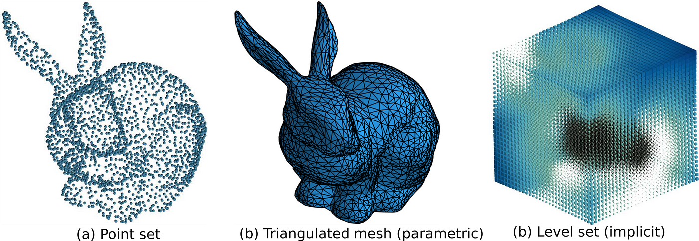
• Implicit: SDF (signed distance field), UDF, NeRF, …

  • continuous
  • easy to decide inside ↔︎ outside
  • hard to sample (rendering) → 결국 explicit form 으로 바꿔야 함

• Explicit: polygonal mesh, occ grid (voxel), Gaussian Splatting, …

  • discreate
  • hard to decide inside ↔︎ outside
  • easy to sample (rendering)

이 중 Mesh 는 explicit representation 의 하나이며, 구체적으로

• $V$: vertex (3D vector)
• $E$: edge (two vertex indices)
• $F$: face (N vertex indices)

의 집합으로 정의된다.

---

B.2. VAE for 3D: vecset-based VAE

이제 3D Generative Model (Shape) 의 학습 목적에 대해 다시 상기해보자.

Diffusion / Flow model 학습보다 선행되는 것은 이 generative model 들을 학습할 잘 정의된 latent space 이다. 2D 에서와 마찬가지로 이러한 latent space 의 필요성은 1) computational cost 의 감소와, 2) semantically meaningful 한 continuous spcae 가 잘 정의되어 있을 때 NN 의 학습이 잘되기 때문이다.

그런 관점에서 3D Mesh 은 VAE 가 latent space 를 학습하기 좋은 domain 이 아니다. VAE 또한 Neural Network 이기 때문에, 고정된 크기의 vector 나 tensor 를 다루는 데 최적화되어 있다. 하지만 Mesh는 어떤가? 모델마다 $V, E, F$의 개수가 제각각이기 때문에 안정적인 학습이 가능한 VAE 의 input/output 으로 설정하는 것이 매우 힘들다.

또한 mesh 자체의 shift / rotation-invaraincy 에 대해서도 생각해볼 수 있다. 어떤 Mesh 가 있을 때 이 Mesh 의 vertices 를 shift/rotation 하면 이는 원본과 다른 객체가 아니다. 즉 Mesh 의 vertices 는 translation/rotation invariance 라고 할 수 있으며, 이를 NN 의 학습 objective 로 삼는 것은 학습이 매우 불안정할 것을 알 수 있다.

따라서 3D Generative Model 의 vecset-based VAE 들은 다음과 같은 설계를 가지고 있다. (figure from 3DShape2vecset)

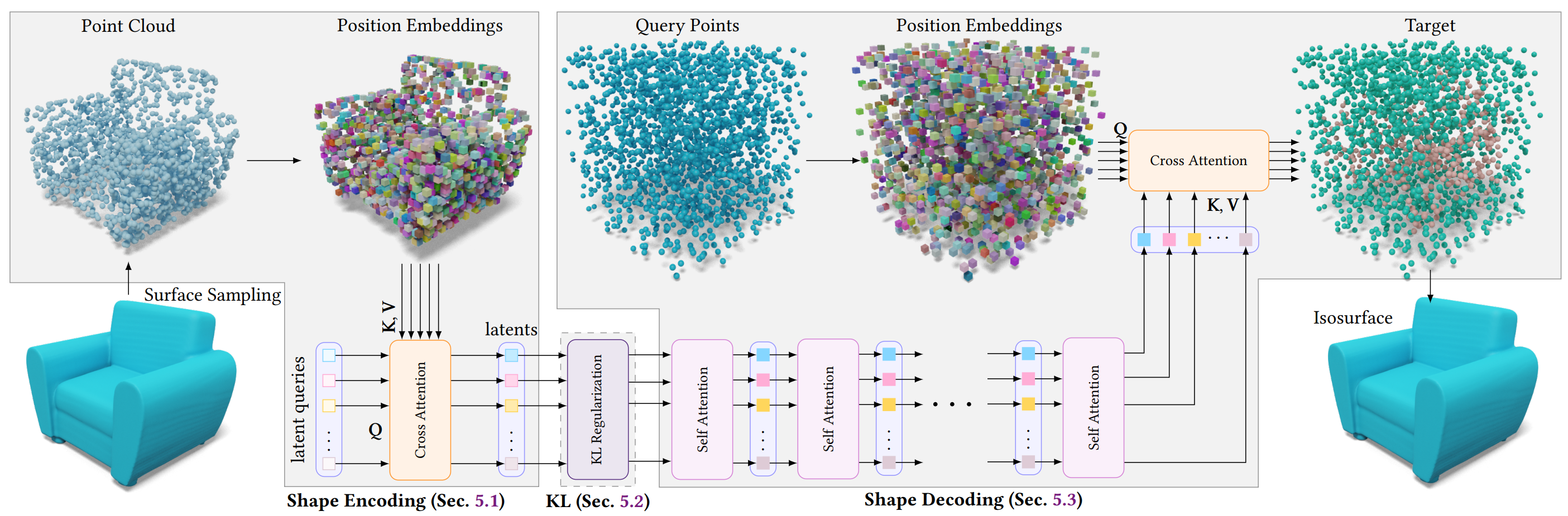
• Input: Mesh 의 surface sampling 한 pointcloud

• Processing: point 에 fourier feature (positional encoding) 을 적용시켜서 NN 이 stationary 한 학습을, point 간 relative relations 에만 집중할 수 있게 해준다. 즉, Mesh 의 translation/rotation invariance 로 인한 ambiguity 를 제거한다. (cf: Fourier Features)

• Training: Pointcloud samples 로부터 VAE encode ↔︎ decode 의 reconstruction 과정을 통해 latent space 를 학습한다. (이 때 kl embedd 로 학습된 bottleneck space 가 Diffusion / Flow 모델의 learnable space 가 된다)

이 과정에서 VAE Decoder 가 mesh representation 대신 output 으로 하는 것이 바로 Implicit Representation, 그중에서도 SDF 나 Occupancy Field 다.

Implicit representation 은 공간 자체를 함수로 정의하기 때문에, VAE decoder 는 latent vector 로부터 SDF 를 근사하는 parametric model 로써 학습된다. 이를 이용해 voxel grid 에서 SDF 를 query 하고 이를 Marching Cube 등을 통해 다시 Mesh 로 복원하는 것 또한 용이하다.

그런데 Implicit Representation의 본질적인 특징은 무엇이었는가? 바로

"Easy to decide inside ↔︎ outside"

라는 것이다.

$$ f(x) = \begin{cases} d(x, \partial \Omega) & \text{if } x \in \Omega \\ -d(x, \partial \Omega) & \text{if } x \in \Omega^c \end{cases} \\ \\ {} \\ \text{where } d(x, \partial \Omega) = \inf_{y \in \partial \Omega} \|x - y\| $$

SDF $f(x)$ 는 표면을 기준으로 내부면 negative, 외부면 positive 값을 갖고, Occupancy는 내부면 1, 외부면 0 을 갖는다. 즉, 이 함수들은 '내부'와 '외부'의 구분이 명확하다는 것을 전제한다.

---

B.3. Watertight Mesh in Mathematics

만약 학습 데이터인 Mesh에 구멍이 뚫려있거나 면이 찢어져 있다면 어떨까? '내부'와 '외부'를 명확히 정의할 수 없게 되고, 이는 SDF의 부호(sign)나 Occupancy의 0/1 값을 결정할 수 없다는 의미다. 이런 모호한 Ground Truth로는 모델이 제대로 학습될 리 없다.

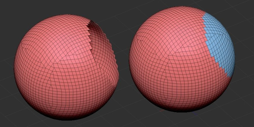
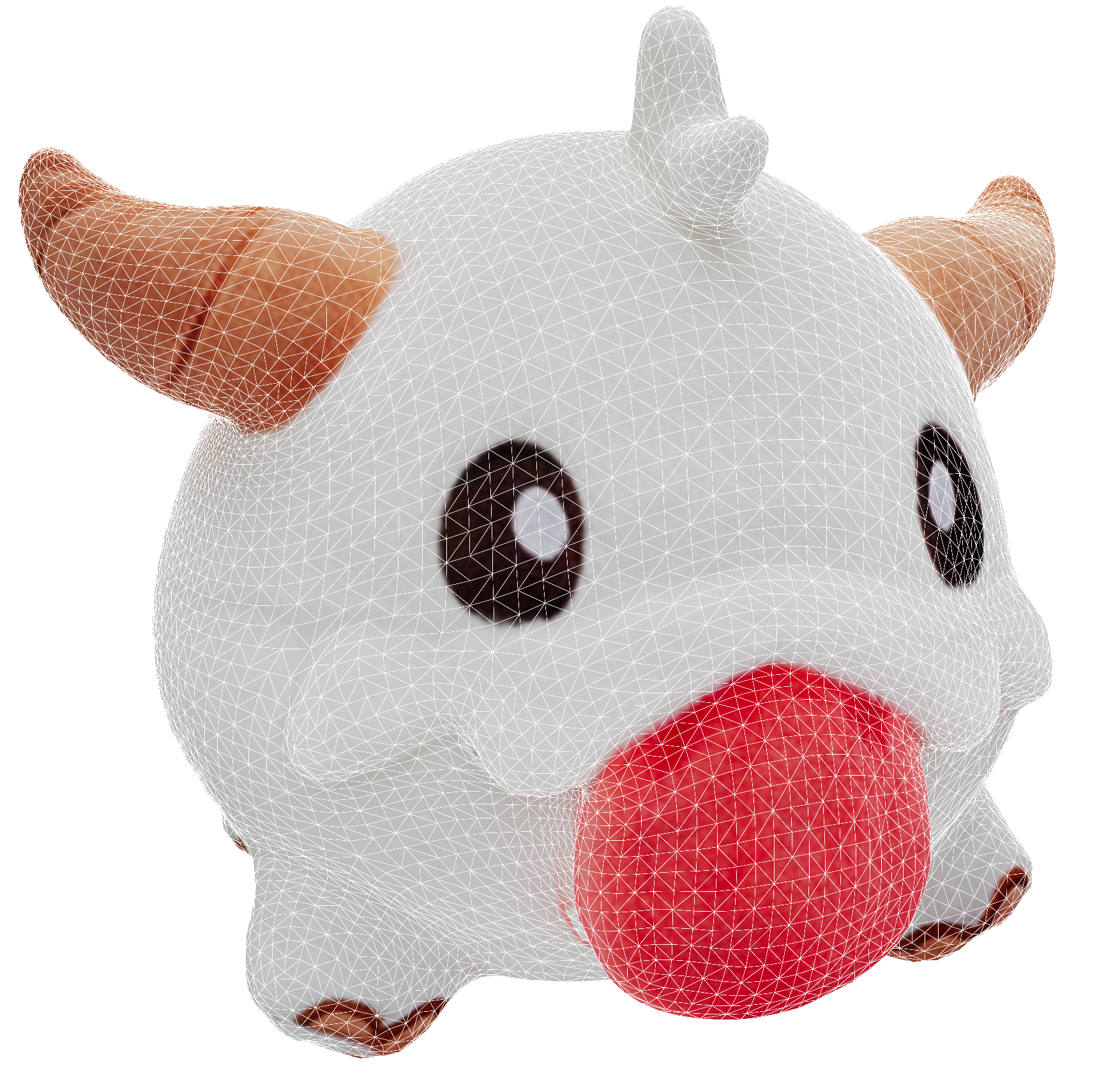
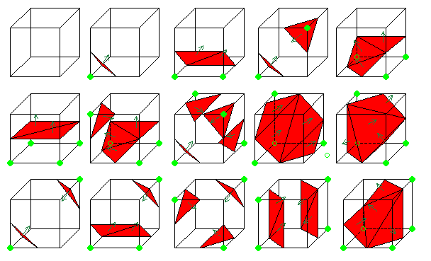
• Fig. Non-Watertight / Watertight

그래서 우리는 모든 Mesh를 '물이 새지 않는', 즉 Watertight 한 상태로 만들어줘야 한다. 이는 수학적으로 다음과 같이 정의된다.

"모든 edge는 정확히 2개의 face에 의해서만 공유된다."

이것은 Mesh가 위상적으로 안정된 2-Manifold 가 되기 위한 최소 조건이다. 2-Manifold 란, surface 의 어떤 점을 확대해도 평평한 2D disk 처럼 보이는 공간을 말한다. (평평이들이 지구를 flat 하다고 생각하는 이유 또한 지구가 2-Manifold 때문이다 :) )

이 개념은 topology 의 핵심인 Euler Characteristic 을 통해 더욱 명확해진다.

닫힌 Manifold, 즉 Watertight Mesh 에 대해서 $V, E, F$ 의 사이에는 항상 다음의 관계가 성립한다.

$$ V - E + F = 2 - 2g $$

(여기서 $g$ 는 Genus 의 개수이다)

• $g=0$ (e.g., Sphere): $V - E + F = 2$

• $g=1$ (e.g. Torus): $V - E + F = 0$

$g=0$ 인 convex manifold 에 대해 $V - E + F = 2$ 임은 잘 알려져 있다 (e.g., 정육면체: $V=8, E=12, F=6$). 여기서 $-2g$ 항이 어떻게 유도되는지, 즉 구멍을 하나 뚫는 과정을 생각해보면 공식을 쉽게 일반화할 수 있다.

1. $g=0$ 인 Watertight Mesh (Euler characteristic = 2) 를 생각해보자.

2. 이 Mesh 표면에서 face 2개를 떼어낸다 ($\triangle F = -2$). Mesh 는 non-watertight 가 되고, $V-E+F$ 값은 2만큼 줄어든다.

3. 이제 뚫린 두 구멍의 경계를 관으로 이어 붙여 다시 Watertight 로 만든다. 이때 추가되는 face 수와 $(n)$ edge 수는 $(n)$ 동일하므로, $V-E+F$ 값은 변하지 않는다 $(\triangle V-\triangle E+ \triangle F = 0-n+n = 0)$.

중요한 것은, 이 공식은 오직 Watertight Mesh 일 때만 성립 한다는 사실이다. Non-watertight Mesh 는 boundary 가 존재하므로 이 공식이 성립하지 않는다.

즉, VAE의 학습 데이터셋에 Watertight 와 Non-watertight 객체가 섞여 있다는 것은, 우리가 보기엔 비슷할지언정 위상적으로 완전히 다른 종류의 객체를 한꺼번에 학습시키는 것과 같다. 이는 VAE가 데이터의 일관된 latent space 를 형성하는 것을 방해하며, 학습을 불안정하게 만든다.

따라서 모든 Mesh에 대한 Watertightness 보장은 안정적인 3D 생성 모델 학습을 위한 가장 근본적인 전처리 과정이라 할 수 있다.

Spatial voxel 을 사용하는 Trellis, Direct3D-S2 등이 거치는 'voxelize' 도 마찬가지이다. activated voxel 을 결정하는 과정은 3D representation 의 topology 에 대한 모호성을 줄여준다. vecset-based VAE 와 spatial voxel-based VAE 를 자세하게 비교하는 글을 이 시리즈 다음 글들에서 좀 더 자세하게 다뤄보도록 하겠다.

---

B.4. How to Make it Watertight: An Algorithmic Deep Dive

자, 이제 우리는 '왜' Watertight Mesh가 필요한지 수학적, 위상학적으로 이해했다. 그럼 남은 질문은 다음과 같다:

'어떻게 non-watertight mesh 를 watertight 하게 만들 것인가?'

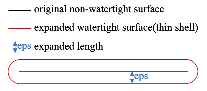
대표적인 Dora 의 구현을 보면, 원본 mesh 전체를 하나의 얇은 닫힌 껍질로 감싸 버리는 알고리즘을 사용한다. (cf: Dora's to_watertightmesh.py)

diffdmc = DiffDMC(dtype=torch.float32).cuda()
vertices, faces = diffdmc(grid_udf, isovalue=eps, normalize= False)

어떤 point 가 Mesh 의 내부인지 외부인지 판별하기는 어려워도, surface 까지의 unsigned distance field (UDF) 를 구하는 것은 쉽기 때문에, 일단 UDF 를 구한 뒤, 원본 surface 로부터 eps 만큼 떨어진 thin shell 을 만들어서, UDF < eps 를 '내부' 로 간주하는, pseudo-isosurface 를 사용하는 것이다. Differentialbe Dual Marching Cube 에 isovalue=eps 가 그것이며, 이로 인해 quantization error 외에도 eps 만큼 original surface 가 dilated, distorted 된 mesh 가 형성된다.

또 다른 방법으로는 UDF (unsigned distance field) 계산 후 flood-fill algorithm 을 사용해 훨씬 robust 하게 watertight mesh 로 변환하는 방법 또한 존재한다. Isovalue 를 non-zero 로 mesh reconstruction 하는 방법과 개념적으로 거의 비슷하지만, 알고리즘 내적으로 어떻게 이를 구현하는지 잘 와닿는 방법이라 해당 방법에 대해 기술하도록 하겠다.

Core Idea: Mesh Reconstruction

기본적으로 이 알고리즘은, 앞서 말했던 original mesh 를 얇은 shell 로 감싸는 알고리즘에 기반한다. 즉, 기존의 불완전한 메쉬를 직접 "수리"하는 방식이 아니다. 대신, 기존의 형태를 본떠서 새로운 watertight mesh 를 reconstruction 하는 방식인 것이다.

Step 1: Voxelization & Unsigned Distance Field

첫 단계는 continuous 3D space 와 가변적인 Mesh 구조를, 우리가 다루기 쉬운 고정된 크기의 Grid 형태로 변환하는 것이다.

resolution = 512
grid_points = torch.stack(
    torch.meshgrid(
        torch.linspace(-1, 1, resolution, device=device),
        torch.linspace(-1, 1, resolution, device=device),
        torch.linspace(-1, 1, resolution, device=device),
        indexing="ij",
    ), dim=-1,
) # [N, N, N, 3]

이후 BVH 를 이용해 이 grid space 에서의 3D 에 대한 unsigned distance field 를 효율적으로 계산하게 된다.

효율적인 BVH 계산을 위한 cubvh Install:

pip install git+https://github.com/ashawkey/cubvh

Python:

vertices = torch.from_numpy(mesh.vertices).float().to(device)
triangles = torch.from_numpy(mesh.faces).long().to(device)

# 2. Build BVH for fast distance query
# using cubvh package!
BVH = cubvh.cuBVH(vertices, triangles)

# 3. Create a voxel grid and query unsigned distance
udf, _, _ = BVH.unsigned_distance(points.view(-1, 3), ...)
udf = udf.view(opt.res, opt.res, opt.res)

여기서 사용하는 cubvh 내부 unsinged_distance_kernel 함수를 일부 살펴보자:

__global__ void unsigned_distance_kernel(
    uint32_t n_elements, const Vector3f* __restrict__ positions,
    float* __restrict__ distances, int64_t* __restrict__ face_id, Vector3f* __restrict__ uvw,
    const TriangleBvhNode* __restrict__ bvhnodes, const Triangle* __restrict__ triangles, bool use_existing_distances_as_upper_bounds
) {
    uint32_t i = blockIdx.x * blockDim.x + threadIdx.x;
    if (i >= n_elements) return;

    float max_distance = use_existing_distances_as_upper_bounds ? distances[i] : MAX_DIST;
    Vector3f point = positions[i];

    // udf result
    auto res = TriangleBvh4::closest_triangle(point, bvhnodes, triangles, max_distance*max_distance);
    distances[i] = res.second;
    face_id[i] = triangles[res.first].id;
}

// C++/CUDA: Inside closest_triangle function
while (!query_stack.empty()) {
    // ...
    // Pruning: if a bounding box is farther than the closest triangle found so far...
    if (children[i].dist <= shortest_distance_sq) {
        query_stack.push(children[i].idx); // ...explore it.
    }
}

• BVH: 모든 점 (Voxel) 과 모든 Face 사이의 거리를 brute-force 로 계산하는 것은 시간이 매우 오래 걸린다. cubvh는 먼저 BVH (Bounding Volume Hierarchy) 라는 tree structure 를 만들어, 거리가 먼 면 그룹 전체를 탐색 후보에서 제외 (Pruning) 함으로써 탐색 성능을 극적으로 향상시킨다. children[i].dist <= shortest_distance_sq

• UDF: CUDA kernel 을 호출하여, GPU의 수많은 thread 에서 병렬로 실행된다. 각 thread 는 voxel point 하나를 맡아, BVH를 통해 가장 가까운 삼각형까지의 Unsigned Distance 를 계산한다.

이 단계가 끝나면, 우리는 원본 메쉬의 형태 정보를 담고 있는 UDF 라는 3D volume data 를 갖게 된다. 하지만 아직 어디가 '내부'이고 어디가 '외부'인지는 모른다.

Step 2: Flood Fill

Flood Fill 알고리즘을 이용하여 내부와 외부를 명확히 구분하게 된다.

Python Code:

# 1. Define the mesh "shell" or "wall"
eps = 2 / opt.res 
occ = udf < eps # Occupancy grid: True if a voxel is on the surface, i.e., make thin shell

# 2. Perform flood fill from an outer corner
#    (internally calls initLabels, hook, compress kernels)
floodfill_mask = cubvh.floodfill(occ)

# 3. Identify all voxels connected to the outside
empty_label = floodfill_mask[0, 0, 0].item()
empty_mask = (floodfill_mask == empty_label)

• Thin Shell (occ = udf < eps): original mesh surface 에 매우 가까운 voxel 들을 True (벽) 로, 나머지를 False (빈 공간) 로 설정하여 메쉬의 "껍질" (shell) 을 만든다. 이 껍질에는 원본의 구멍이나 틈이 그대로 반영되어 있을 수 있다. (구멍의 크기가 eps 보다 작다면 무시될 것이다)

cubvh's floodfill kernel:

// C++/CUDA: Inside hook kernel
int best = labels[idx];
// ... check 6 neighbors ...
// idx +- 1, idx +- W, idx +- W*H
if (x > 0 && grid[idx-1]==0) best = min(best, labels[idx-1]);
// ... (5 more neighbors)

if (best < labels[idx]) {
    labels[idx] = best;
    atomicOr(changed, 1); // Mark that a change occurred
}

(Labeling & Spread)

• 모든 voxel grid 에 고유한 ID 를 부여한다.

• hook & compress: 격자의 모서리 $[0,0,0]$ (명백한 외부) 에서부터 "물"을 채우기 시작 한다. 각 "빈 공간" Voxel은 주변 이웃의 (6 neighbors) 레이블을 확인하고, _가장 작은 값으로 자신의 레이블을 업데이트 . 이 과정은 "벽" (occ=True) 을 통과하지 못하며, compress 커널 (pointer jumping)을 통해 전파 속도를 가속화한다.

• 최종 판별: 모든 전파가 끝나면, [0,0,0] 과 같은 레이블을 가진 모든 Voxel은 '외부 공간'으로 확정된다 (empty_mask).

즉 Mesh 가 정의된 canonical space 의 외곽에서부터 일종의 '물을 흘려보내는 simulation' 을 실행하는 것과 같다. 이를 통해 Non-watertight 메쉬의 구멍이나 틈이 occ 껍질에 의해 자연스럽게 "메워지고", Flood Fill을 통해 내부와 외부가 완벽하게 분리된 볼륨 데이터를 얻는다.

Step 3: Signed Distance Field

이제 UDF를 Marching Cubes가 사용할 수 있는 SDF로 변환한다.

Python Code:

# 1. Invert the empty mask to get inside + shell
occ_mask = ~empty_mask

# 2. Initialize SDF: surface is 0, outside is positive
sdf = udf - eps

# 3. Assign negative sign to the inside
inner_mask = occ_mask & (sdf > 0)
sdf[inner_mask] *= -1

• occ_mask는 '벽 (shell)'과 Flood Fill에서 '외부'로 판명되지 않은 '진정한 내부' 를 모두 포함한다.

• sdf = udf - eps를 통해 표면 근처의 값을 0으로 맞춘다.

• occ_mask 를 이용해 내부에 해당하는 Voxel들의 SDF 값에 -1을 곱해 음수로 만든다.

결과적으로, sdf는 내부는 음수, 외부는 양수, 표면은 0의 값을 갖는 완벽한 Signed Distance Field 가 된다.

Step 4: Marching Cubes

마지막으로, 이 완벽한 SDF 볼륨 데이터로부터 새로운 Watertight 메쉬를 추출한다.

Python Code:

# 1. Extract the iso-surface where sdf = 0
vertices, triangles = mcubes.marching_cubes(sdf, 0)

# 2. Normalize vertices and convert to a trimesh object
vertices = vertices / (opt.res - 1.0) * 2 - 1
watertight_mesh = trimesh.Trimesh(vertices, triangles)

# 3. Restore original scale and save
watertight_mesh.vertices = watertight_mesh.vertices * original_radius + original_center
watertight_mesh.export(f'{opt.workspace}/{name}.obj')

Marching Cubes 알고리즘은 3D 격자 데이터 (SDF) 를 입력받아, SDF 값이 0이 되는 지점 (isosurface)을 찾아 삼각형 메쉬로 만들어준다. 이 알고리즘의 출력물은 그 정의상 항상 닫힌 표면, 즉 Watertight이다.

---

B.5. Pointcloud Sampling

이제 watertight conversion 이 완료되었으므로, mesh 에 대한 pre-processing 단계의 마지막 부분은 오로지 pointcloud sampling 뿐이다. mesh surface 위에서 uniform 하게 point 를 뽑는 것은 어렵지 않으나, 최근 Dora, Hunyuan3D, TripoSG 등은 salient edge, 즉 특징적인 모서리에서 point 를 더 많이 뽑는 것이 VAE reconstruction 성능에 훨씬 도움된다는 report 를 한 바 있다.

SES sampling 자체는 Dora github 에 구현되어 제공되기는 하는데, 이 과정에서 Blender 설치와 bpy 가 필요해서 sampling 과정 자체가 무거워진다.

따라서 이 아래에서는, blender 의 기능을 사용하는 대신 pure python 으로 salient edge sampling 을 구현해보도록 하겠다.

Step 1: Salient Edge

• Assumption: "Salient edge"는 edge 를 공유하는 두 face 이 이루는 Dihedral Angle 가 큰 edge 일 것이다.

즉 우리는 Mesh 에서 서로 인접한 face 간의 normal vector 의 dot product 를 이용하여 certain threshold 보다 큰 ‘Salient edge’ 를 판별할 수 있다.

salient_edges = []
total_edge_length = 0.0

# mesh.edges_unique: corners (v1_idx, v2_idx)
for i, face_pair in enumerate(mesh.face_adjacency):
    face1_idx, face2_idx = face_pair
    normal1 = mesh.face_normals[face1_idx]
    normal2 = mesh.face_normals[face2_idx]
    
    angle = np.arccos(np.clip(np.dot(normal1, normal2), -1.0, 1.0))

    if angle > thresh_angle_rad:
        edge_vertices_indices = mesh.face_adjacency_edges[i]
        v1_idx, v2_idx = edge_vertices_indices
        
        v1 = mesh.vertices[v1_idx]
        v2 = mesh.vertices[v2_idx]
        length = np.linalg.norm(v1 - v2)
        
        if length > 1e-8:
            total_edge_length += length
            salient_edges.append((v1_idx, v2_idx, length))

위와 같이 두 normal vector 의 dot product 를 구하고 arccos 함수를 적용하여 사이각을 계산한다.

Step 2: Init Sampling

이후 Sampling 의 첫 단계는, salient edge 의 양 끝 vertex 를 sampling 하는 것이다. step 1 에서 찾은 salient_edges 리스트를 순회하며 각 모서리의 시작점 (v1_idx)과 끝점 (v2_idx) 인덱스를 가져와서 init samples 로 활용한다.

initial_samples = []
added_vertex_indices = set()
for v1_idx, v2_idx, _ in salient_edges:
    if v1_idx not in added_vertex_indices:
        initial_samples.append(mesh.vertices[v1_idx])
        added_vertex_indices.add(v1_idx)
    if v2_idx not in added_vertex_indices:
        initial_samples.append(mesh.vertices[v2_idx])
        added_vertex_indices.add(v2_idx)

samples = np.array(initial_samples)

Step 3: Interpolation

2단계에서 수집한 꼭짓점의 수가 목표한 sampling 보다 적을 수 있기 때문에, salient edge 위에서 points 를 추가적으로 Sampling 한다. 이 때, 긴 모서리가 짧은 모서리보다 더 많은 특징을 담고 있다고 가정하고, 모서리의 길이에 비례 하여 추가할 샘플의 개수를 할당하여 sampling 한다.

num_extra = num_samples - len(samples)
extra_samples = []
if total_edge_length > 0:
    for v1_idx, v2_idx, length in salient_edges:
        # based on the edge length, proportionally distribute extra samples
        extra_this_edge = math.ceil(num_extra * length / total_edge_length)
        
        v1 = mesh.vertices[v1_idx]
        v2 = mesh.vertices[v2_idx]
        
        for j in range(extra_this_edge):
            t = (j + 1.0) / (extra_this_edge + 1.0)
            new_point = v1 + (v2 - v1) * t
            extra_samples.append(new_point)

이 때, 한 edge 안에서 균등한 sampling 을 위해 linear interpolation 을 이용한다.

Final Step

이제 마지막으로 FPS (Farthest Point Sampling) 를 이용해서 목표 sample 수와 정확하게 맞춰준다. 정확히 num_samples 개의 점을 선택한다.

Furthest Point Sampling package Install:

pip install fpsample

python:

if len(all_samples) > num_samples:
    indices = fpsample.bucket_fps_kdline_sampling(all_samples, num_samples, h=5)
    return all_samples[indices]

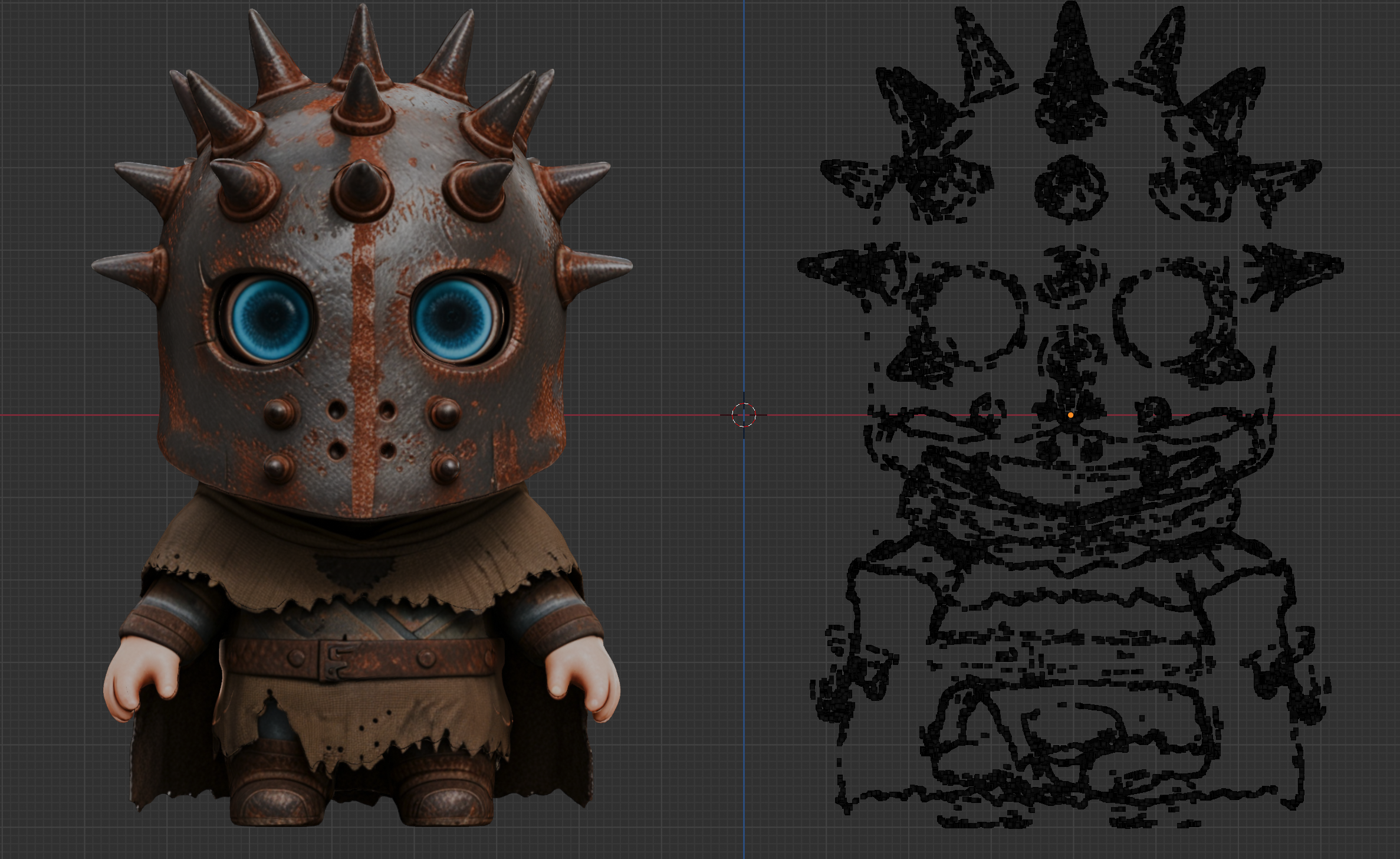
• Result (Left: Input Mesh, Right: Output Salient Sampling ptc)

정상적으로 동작하는 개념적인 구현이긴 하지만, c++ 로 구현되어 훨씬 빠르게 sampling 할 수 있는 meshiki 패키지가 있으니, 이를 이용하면 다음과 같이 ses 를 바로 구현할 수 있다.

# pip install meshiki
from meshiki import Mesh, fps, load_mesh, triangulate

vertices, faces = load_mesh(mesh_path, clean=True)
faces = triangulate(faces)
mesh = Mesh(vertices, faces)

# sample 64K salient points
salient_points = mesh.salient_point_sample(64000, thresh_bihedral=30)

---

마치며

이번 글에서는 3D Generative Model 을 구축하기 위한 첫걸음, data pre-processing 에 대해서 심도 깊게 다뤄보았다.

위에서 다룬 processing 뿐만 아니라 실제로는 mesh 에 대한 multi-view rendering 까지 진행해야하기 때문에, 추가적으로 bpy 를 활용한 Blender rendering script 까지 다룰 수 있어야 3D Generative Model 에 대한 pre-processing 을 완벽하게 구사할 수 있다 말할 수 있겠다. (cf: Blenderproc, Trellis dataset toolkits)

3D Generative Model 또한 LLM 만큼은 아니어도 3D Generative Model 또한 최소 1B~3B 정도의 model 을 학습하기 위해 VRAM 80G 이상의 GPU 최소 64개, 3D data 처리로 인한 20T 이상의 NAS 등이 필요한 cost-consuming task 이다.

하지만 open source 로도 훌륭한 모델들이 계속해서 공급되고 있고, 이러한 모델을 이용해 가장 비싼 자원인 GPU 를 적게 쓰면서도 공개되는 foundation model 에 대한 finetuning, LoRA-Adapter Training 등을 위해서라면 적어도 3D data 에 대한 pre-processing 은 필수적으로 다룰 수 있어야 한다.

필자는 작년 CaPa Project 를 진행한 이후로 자체 3D 생성 모델을 학습시키고, 이를 기반으로하는 3D 생성 서비스를 개발 중에 있다. 곧 사외 공개 예정이 있으니 이를 소개할 수 있으면 좋을 것 같다.

이 시리즈의 다음 글에서는 본격적인 ShapeVAE, Flow Model Structure 분석 등과, training 에 필요한 multi-node 환경을 구축하고 Deepspeed v3, FSDP 의 sharding 전략을 사용하여 3D Generative Model 을 효율적으로 학습시키기 위한 전략 등에 대해 다뤄볼 예정이다.

Stay Tuned!

---

You may also likes

• 3D 생성에서 NeRF 와 SDS 는 도태될 수밖에 없는가? (velog)
• 3D 생성 모델의 시대